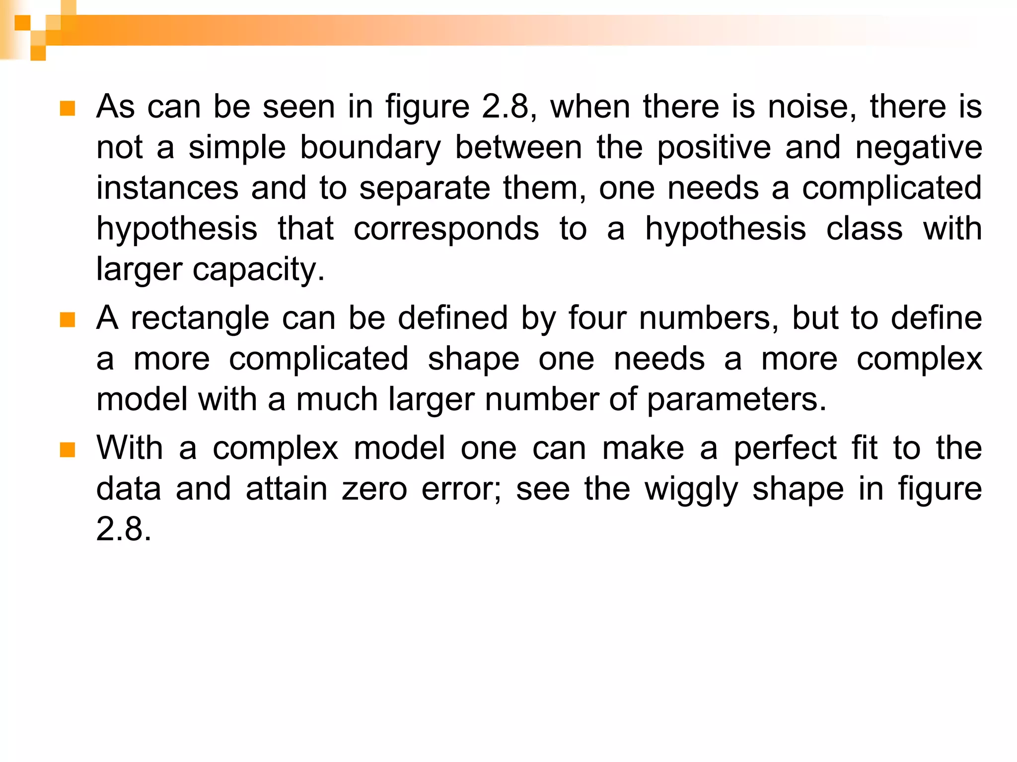
SlideShare a Scribd company logo
CHAPTER 2:
Supervised Learning
Machine Learning
 Machine learning is a subset of AI, which enables the
machine to automatically learn from data, improve
performance from past experiences, and make
predictions.
 Machine learning contains a set of algorithms that work on
a huge amount of data.
 Data is fed to these algorithms to train them, and on the
basis of training, they build the model & perform a specific
task.
 These ML algorithms help to solve different business
problems like Regression, Classification, Forecasting,
Clustering, and Associations, etc.
 Based on the methods and way of learning,
machine learning is divided into mainly four types,
which are:
 Supervised Machine Learning
 Unsupervised Machine Learning
 Semi-Supervised Machine Learning
 Reinforcement Learning
Types of Machine Learning
Outline of this chapter
 Learning a Class from Examples,
 Vapnik-Chervonenkis Dimension,
 Probably Approximately Correct Learning,
 Noise,
 Learning Multiple Classes,
 Regression,
 Model Selection and Generalization,
 Dimensions of a Supervised Machine Learning Algorithm
Learning a Class from Examples
 Let us say we want to learn the class, C, of a “family
car.”
 We have a set of examples of cars, and we have a
group of people that we survey to whom we show
these cars.
 The people look at the cars and label them; the cars
that they believe are family cars are positive
examples, and the other cars are negative examples.
 Class learning is finding a description that is shared
by all the positive examples and none of the negative
examples.
 Doing this, we can make a prediction: Given a car that we
have not seen before, by checking with the description
learned, we will be able to say whether it is a family car or
not.
 Or we can do knowledge extraction: This study may be
sponsored by a car company, and the aim may be to
understand what people expect from a family car.
 After some discussions with experts in the field, let us say
that we reach the conclusion that among all features a car
may have, the features that separate a family car from
other type of cars are the price and engine power.
 These two attributes are the inputs to the class recognizer.
 Note that when we decide on this particular input
representation, we are ignoring various other attributes as
irrelevant.
 Though one may think of other attributes such as seating
capacity and color that might be important for distinguishing
among car types, we will consider only price and engine
power to keep this example simple.
 Class C of a “family car”
 Prediction: Is car x a family car?
 Knowledge extraction: What do people expect from a
family car?
 Input representation:
x1: price, x2 : engine power
 Output:
Positive (+) and negative (–) examples
 Training set for the class of a “family car.”
 Each data point corresponds to one example car, and the
coordinates of the point indicate the price and engine
power of that car.
 ‘+’ denotes a positive example of the class (a family car),
and
 ‘−’ denotes a negative example (not a family car); it is
another type of car.
 Let us denote price as the first input attribute x1 and
engine power as the second attribute x2 .
 Thus we represent each car using two numeric values
 Our training data can now be plotted in the two-dimensional
(x1, x2) space where each instance t is a data point at
coordinates and its type, namely, positive versus
negative, is given by
 After further discussions with the expert and the analysis of
the data, we may have reason to believe that for a car to be
a family car, its price and engine power should be in a
certain range.
(p1 ≤ price ≤ p2) AND (e1 ≤ engine power ≤ e2)
for suitable values of p1, p2, e1, and e2.
 The above equation fixes H, the hypothesis class from which we
believe C is drawn, namely, the set of rectangles.
 The learning algorithm then finds hypothesis the particular
hypothesis, h ∈ H, specified by a particular quadruple of (ph1, ph2,
eh1, eh2), to approximate C as closely as possible.
Training set X N
t
t
t
,r 1
}
{ 
 x
X




negative
is
if
0
positive
is
if
1
x
x
r







2
1
x
x
x
Class C
   
2
1
2
1 power
engine
AND
price e
e
p
p 



Hypothesis class H




negative
as
classifies
if
0
positive
as
classifies
if
1
)
(
x
x
x
h
h
h
Error of h on H
 
 




N
t
t
t
r
h
h
E
1
1
)
|
( x
X
S, G, and the Version Space
most specific hypothesis, S
most general hypothesis, G
h  H, between S and G is
consistent
and make up the
version space
(Mitchell, 1997)
 One possibility is to find the most specific hypothesis, S,
that is the tightest rectangle that includes all the positive
examples and none of the negative examples.
 The most general hypothesis, G, is the largest rectangle
we can draw that includes all the positive examples and
none of the negative examples.
 Any h∈H between S and G is a valid hypothesis with no
error, said to be consistent with the training set, and such h
make up the version space.
Candidate Elimination Algorithm
 The candidate elimination algorithm incrementally builds the
version space given a hypothesis space H and a set E of
examples.
 The examples are added one by one; each example
possibly shrinks the version space by removing the
hypotheses that are inconsistent with the example.
 The candidate elimination algorithm does this by updating
the general and specific boundary for each new example.
Terms Used:
Concept learning:
• Concept learning is basically learning task of the machine
(Learn by Train data)
General Hypothesis:
• Not Specifying features to learn the machine.
• G = {‘?’, ‘?’,’?’,’?’…}: Number of attributes
Specific Hypothesis:
• Specifying features to learn machine (Specific feature)
• S= {‘pi’,’pi’,’pi’…}: Number of pi depends on number of
attributes.
Version Space:
• It is intermediate of general hypothesis and Specific
hypothesis.
Algorithm:
Step1: Load Data set
Step2: Initialize General Hypothesis and Specific Hypothesis.
Step3: For each training example
Step4: If example is positive example
if attribute_value == hypothesis_value:
Do nothing
else:
replace attribute value with '?’
(Basically generalizing it)
Step5: If example is Negative example
Make generalize hypothesis more specific.
Example:
 Consider the dataset given below:
Sky Temperature Humid Wind Water Forest Output
Sunny Warm Normal Strong Warm Same Yes
Sunny Warm High Strong Warm Same Yes
Rainy Cold High Strong Warm Change No
Sunny Warm High Strong Cool Change Yes
Algorithmic steps:
Initially :
G = [[?, ?, ?, ?, ?, ?], [?, ?, ?, ?, ?, ?], [?, ?, ?, ?, ?, ?],
[?, ?, ?, ?, ?, ?], [?, ?, ?, ?, ?, ?], [?, ?, ?, ?, ?, ?]]
S = [Null, Null, Null, Null, Null, Null]
For instance 1 :
<'sunny','warm','normal','strong','warm ','same’>
and positive output.
G1 = G
S1 = ['sunny','warm','normal','strong','warm ','same']
For instance 2 :
<'sunny','warm','high','strong','warm ','same’>
and positive output.
G2 = G
S2 = ['sunny','warm',?,'strong','warm ','same’]
For instance 3 :
<'rainy','cold','high','strong','warm ','change’>
and negative output.
G3 = [['sunny', ?, ?, ?, ?, ?], [?, 'warm', ?, ?, ?, ?],
[?, ?, ?, ?, ?, ?], [?, ?, ?, ?, ?, ?], [?, ?, ?, ?, ?, ?],
[?, ?, ?, ?, ?, 'same']]
S3 = S2
For instance 4 : <'sunny','warm','high','strong','cool','change’>
and positive output.
G4 = G3
S4 = ['sunny','warm',?,'strong', ?, ?]
 At last, by synchronizing the G4 and S4 algorithm produce
the output.
Output :
 G = [['sunny', ?, ?, ?, ?, ?], [?, 'warm', ?, ?, ?, ?]]
 S = ['sunny','warm',?,'strong', ?, ?]
Vapnik-Chervonenkis Dimension
 Let us say we have a dataset containing N points.
 These N points can be labeled in 2N ways as positive and
negative.
 Therefore, 2N different learning problems can be defined by
N data points.
 If for any of these problems, we can find a hypothesis h∈H
that separates the positive examples from the negative,
then we say H shatters N points.
 That is, any learning problem definable by N examples can
be learned with no error by a hypothesis drawn from H.
 The maximum number of points that VC dimension can be
shattered by H is called the Vapnik-Chervonenkis (VC)
dimension of H, is denoted as VC(H), and measures the
capacity of H.
VC Dimension
 N points can be labeled in 2N ways as +/–
 H shatters N if there
exists h  H consistent
for any of these:
VC(H ) = N
An axis-aligned rectangle shatters 4 points only !
 How many training examples N should we have, such that with
probability at least 1 ‒ δ, h has error at most ε ?
(Blumer et al., 1989)
 Each strip is at most ε/4
 Pr that we miss a strip 1‒ ε/4
 Pr that N instances miss a strip (1 ‒ ε/4)N
 Pr that N instances miss 4 strips 4(1 ‒ ε/4)N
 4(1 ‒ ε/4)N ≤ δ and (1 ‒ x)≤exp( ‒ x)
 4exp(‒ εN/4) ≤ δ and N ≥ (4/ε)log(4/δ)
Probably Approximately Correct
(PAC) Learning
Noise
 Noise is any
unwanted
anomaly in the
data and due to
noise, the class
may be more
difficult to learn
and zero error
may be
infeasible with a
simple
hypothesis
class. (see
figure 2.8)
 There are several interpretations of noise:
 There may be imprecision in recording the input attributes, which
may shift the data points in the input space.
 There may be errors in labeling the data points, which may relabel
positive instances as negative and vice versa. This is sometimes
called teacher noise.
 There may be additional attributes, which we have not taken into
account, that affect the label of an instance. Such attributes may
be hidden or latent in that they may be unobservable. The effect of
these neglected attributes is thus modeled as a random
component and is included in “noise.”
 As can be seen in figure 2.8, when there is noise, there is
not a simple boundary between the positive and negative
instances and to separate them, one needs a complicated
hypothesis that corresponds to a hypothesis class with
larger capacity.
 A rectangle can be defined by four numbers, but to define
a more complicated shape one needs a more complex
model with a much larger number of parameters.
 With a complex model one can make a perfect fit to the
data and attain zero error; see the wiggly shape in figure
2.8.
31
Use the simpler one because
 Simpler to use
(lower computational
complexity)
 Easier to train (lower
space complexity)
 Easier to explain
(more interpretable)
 Generalizes better (lower
variance - Occam’s razor)
Noise and Model Complexity
Learning Multiple Classes
 In our example of learning a family car, we have positive
examples belonging to the class family car and the
negative examples belonging to all other cars.
 This is a two-class problem.
 In the general case, we have K classes denoted as Ci, i =
1, . . . , K, and an input instance belongs to one and
exactly one of them.
Multiple Classes, Ci i=1,...,K
N
t
t
t
,r 1
}
{ 
 x
X









,
if
0
if
1
i
j
r
j
t
i
t
t
i
C
C
x
x
Train hypotheses
hi(x), i =1,...,K:
 









,
if
0
if
1
i
j
h
j
t
i
t
t
i
C
C
x
x
x
 In machine learning for classification, we would like to
learn the boundary separating the instances of one class
from the instances of all other classes.
 Thus we view a K-class classification problem as K two-
class problems.
 The training examples belonging to Ci are the positive
instances of hypothesis hi and the examples of all other
classes are the negative instances of hi.
 The total empirical error takes a sum over the predictions
for all classes over all instances:
Regression
 In classification, given an input, the output that is
generated is Boolean; it is a yes/no answer.
 When the output is a numeric value, what we would like
to learn is not a class, C(x) ∈ {0, 1}, but is a numeric
function.
 In machine learning, the function is not known but we
have a training set of examples drawn from it
Regression   0
1 w
x
w
x
g 

  0
1
2
2 w
x
w
x
w
x
g 


   
 




N
t
t
t
x
g
r
N
g
E
1
2
1
| X
   
 





N
t
t
t
w
x
w
r
N
w
,
w
E
1
2
0
1
0
1
1
| X
 
  




 
t
t
t
N
t
t
t
x
f
r
r
r
x 1
,
X
Model Selection & Generalization
 Learning is an ill-posed problem; data is not sufficient to
find a unique solution
 The need for inductive bias, assumptions about H
 Generalization: How well a model performs on new data
 Overfitting: H more complex than C or f
 Underfitting: H less complex than C or f
Triple Trade-Off
 There is a trade-off between three factors (Dietterich,
2003):
1. Complexity of H, c (H),
2. Training set size, N,
3. Generalization error, E, on new data
 As N, E
 As c (H), first E and then E
Cross-Validation
 To estimate generalization error, we need data unseen
during training. We split the data as
 Training set (50%)
 Validation set (25%)
 Test (publication) set (25%)
 Resampling when there is few data
Dimensions of a Supervised
Learner
1. Model :
2. Loss function:
3. Optimization procedure:
 

|
x
g
   
 
 


t
t
t
g
,
r
L
E |
| x
X
 
X
|
min
arg 



E
*

More Related Content

What's hot

Stacking ensemble
Stacking ensembleStacking ensemble
Stacking ensemble
kalung0313
 
Face recognition using PCA
Face recognition using PCAFace recognition using PCA
Face recognition using PCA
Nawin Kumar Sharma
 
Medical image analysis
Medical image analysisMedical image analysis
Medical image analysis
Aboul Ella Hassanien
 
Design cycles of pattern recognition
Design cycles of pattern recognitionDesign cycles of pattern recognition
Design cycles of pattern recognition
Al Mamun
 
House Price Prediction An AI Approach.
House Price Prediction An AI Approach.House Price Prediction An AI Approach.
House Price Prediction An AI Approach.
Nahian Ahmed
 
Breast cancer Detection using MATLAB
Breast cancer Detection using MATLABBreast cancer Detection using MATLAB
Breast cancer Detection using MATLAB
NupurRathi7
 
Ensemble methods in machine learning
Ensemble methods in machine learningEnsemble methods in machine learning
Ensemble methods in machine learning
SANTHOSH RAJA M G
 
Introduction to Machine Learning
Introduction to Machine LearningIntroduction to Machine Learning
Introduction to Machine Learning
Panimalar Engineering College
 
Lecture 4 Decision Trees (2): Entropy, Information Gain, Gain Ratio
Lecture 4 Decision Trees (2): Entropy, Information Gain, Gain RatioLecture 4 Decision Trees (2): Entropy, Information Gain, Gain Ratio
Lecture 4 Decision Trees (2): Entropy, Information Gain, Gain Ratio
Marina Santini
 
Linear Regression Algorithm | Linear Regression in Python | Machine Learning ...
Linear Regression Algorithm | Linear Regression in Python | Machine Learning ...Linear Regression Algorithm | Linear Regression in Python | Machine Learning ...
Linear Regression Algorithm | Linear Regression in Python | Machine Learning ...
Edureka!
 
Clustering:k-means, expect-maximization and gaussian mixture model
Clustering:k-means, expect-maximization and gaussian mixture modelClustering:k-means, expect-maximization and gaussian mixture model
Clustering:k-means, expect-maximization and gaussian mixture model
jins0618
 
House Sale Price Prediction
House Sale Price PredictionHouse Sale Price Prediction
House Sale Price Prediction
sriram30691
 
Classification using back propagation algorithm
Classification using back propagation algorithmClassification using back propagation algorithm
Classification using back propagation algorithm
KIRAN R
 
Machine learning
Machine learningMachine learning
Machine learning
Sanjay krishne
 
Supervised Machine Learning With Types And Techniques
Supervised Machine Learning With Types And TechniquesSupervised Machine Learning With Types And Techniques
Supervised Machine Learning With Types And Techniques
SlideTeam
 
2.mathematics for machine learning
2.mathematics for machine learning2.mathematics for machine learning
2.mathematics for machine learning
KONGU ENGINEERING COLLEGE
 
Classification and Regression
Classification and RegressionClassification and Regression
Classification and Regression
Megha Sharma
 
Machine Learning With Logistic Regression
Machine Learning  With Logistic RegressionMachine Learning  With Logistic Regression
Machine Learning With Logistic Regression
Knoldus Inc.
 
Introduction To Machine Learning
Introduction To Machine LearningIntroduction To Machine Learning
Introduction To Machine Learning
Knoldus Inc.
 
Breast cancer detection using Artificial Neural Network
Breast cancer detection using Artificial Neural NetworkBreast cancer detection using Artificial Neural Network
Breast cancer detection using Artificial Neural Network
Subroto Biswas
 

What's hot (20)

Stacking ensemble
Stacking ensembleStacking ensemble
Stacking ensemble
 
Face recognition using PCA
Face recognition using PCAFace recognition using PCA
Face recognition using PCA
 
Medical image analysis
Medical image analysisMedical image analysis
Medical image analysis
 
Design cycles of pattern recognition
Design cycles of pattern recognitionDesign cycles of pattern recognition
Design cycles of pattern recognition
 
House Price Prediction An AI Approach.
House Price Prediction An AI Approach.House Price Prediction An AI Approach.
House Price Prediction An AI Approach.
 
Breast cancer Detection using MATLAB
Breast cancer Detection using MATLABBreast cancer Detection using MATLAB
Breast cancer Detection using MATLAB
 
Ensemble methods in machine learning
Ensemble methods in machine learningEnsemble methods in machine learning
Ensemble methods in machine learning
 
Introduction to Machine Learning
Introduction to Machine LearningIntroduction to Machine Learning
Introduction to Machine Learning
 
Lecture 4 Decision Trees (2): Entropy, Information Gain, Gain Ratio
Lecture 4 Decision Trees (2): Entropy, Information Gain, Gain RatioLecture 4 Decision Trees (2): Entropy, Information Gain, Gain Ratio
Lecture 4 Decision Trees (2): Entropy, Information Gain, Gain Ratio
 
Linear Regression Algorithm | Linear Regression in Python | Machine Learning ...
Linear Regression Algorithm | Linear Regression in Python | Machine Learning ...Linear Regression Algorithm | Linear Regression in Python | Machine Learning ...
Linear Regression Algorithm | Linear Regression in Python | Machine Learning ...
 
Clustering:k-means, expect-maximization and gaussian mixture model
Clustering:k-means, expect-maximization and gaussian mixture modelClustering:k-means, expect-maximization and gaussian mixture model
Clustering:k-means, expect-maximization and gaussian mixture model
 
House Sale Price Prediction
House Sale Price PredictionHouse Sale Price Prediction
House Sale Price Prediction
 
Classification using back propagation algorithm
Classification using back propagation algorithmClassification using back propagation algorithm
Classification using back propagation algorithm
 
Machine learning
Machine learningMachine learning
Machine learning
 
Supervised Machine Learning With Types And Techniques
Supervised Machine Learning With Types And TechniquesSupervised Machine Learning With Types And Techniques
Supervised Machine Learning With Types And Techniques
 
2.mathematics for machine learning
2.mathematics for machine learning2.mathematics for machine learning
2.mathematics for machine learning
 
Classification and Regression
Classification and RegressionClassification and Regression
Classification and Regression
 
Machine Learning With Logistic Regression
Machine Learning  With Logistic RegressionMachine Learning  With Logistic Regression
Machine Learning With Logistic Regression
 
Introduction To Machine Learning
Introduction To Machine LearningIntroduction To Machine Learning
Introduction To Machine Learning
 
Breast cancer detection using Artificial Neural Network
Breast cancer detection using Artificial Neural NetworkBreast cancer detection using Artificial Neural Network
Breast cancer detection using Artificial Neural Network
 

Similar to Supervised_Learning.ppt

AML_030607.ppt
AML_030607.pptAML_030607.ppt
AML_030607.ppt
butest
 
Essentials of machine learning algorithms
Essentials of machine learning algorithmsEssentials of machine learning algorithms
Essentials of machine learning algorithms
Arunangsu Sahu
 
Machine Learning
Machine LearningMachine Learning
Machine Learning
butest
 
introducción a Machine Learning
introducción a Machine Learningintroducción a Machine Learning
introducción a Machine Learning
butest
 
introducción a Machine Learning
introducción a Machine Learningintroducción a Machine Learning
introducción a Machine Learning
butest
 
Alpaydin - Chapter 2
Alpaydin - Chapter 2Alpaydin - Chapter 2
Alpaydin - Chapter 2
butest
 
Alpaydin - Chapter 2
Alpaydin - Chapter 2Alpaydin - Chapter 2
Alpaydin - Chapter 2
butest
 
Lecture 7
Lecture 7Lecture 7
Lecture 7
butest
 
Lecture 7
Lecture 7Lecture 7
Lecture 7
butest
 
ppt
pptppt
ppt
butest
 
ML_ Unit_1_PART_A
ML_ Unit_1_PART_AML_ Unit_1_PART_A
ML_ Unit_1_PART_A
Srimatre K
 
Lecture 3 (Supervised learning)
Lecture 3 (Supervised learning)Lecture 3 (Supervised learning)
Lecture 3 (Supervised learning)
VARUN KUMAR
 
Deep Learning: Introduction & Chapter 5 Machine Learning Basics
Deep Learning: Introduction & Chapter 5 Machine Learning BasicsDeep Learning: Introduction & Chapter 5 Machine Learning Basics
Deep Learning: Introduction & Chapter 5 Machine Learning Basics
Jason Tsai
 
Machine Learning and Inductive Inference
Machine Learning and Inductive InferenceMachine Learning and Inductive Inference
Machine Learning and Inductive Inference
butest
 
Machine Learning: Decision Trees Chapter 18.1-18.3
Machine Learning: Decision Trees Chapter 18.1-18.3Machine Learning: Decision Trees Chapter 18.1-18.3
Machine Learning: Decision Trees Chapter 18.1-18.3
butest
 
Midterm
MidtermMidterm
Machine learning and_nlp
Machine learning and_nlpMachine learning and_nlp
Machine learning and_nlp
ankit_ppt
 
Understanding Blackbox Prediction via Influence Functions
Understanding Blackbox Prediction via Influence FunctionsUnderstanding Blackbox Prediction via Influence Functions
Understanding Blackbox Prediction via Influence Functions
SEMINARGROOT
 
Candidate elimination algorithm in ML Lab
Candidate elimination algorithm in ML LabCandidate elimination algorithm in ML Lab
Candidate elimination algorithm in ML Lab
VenkateswaraBabuRavi
 
Lecture 3.1_ Logistic Regression.pptx
Lecture 3.1_ Logistic Regression.pptxLecture 3.1_ Logistic Regression.pptx
Lecture 3.1_ Logistic Regression.pptx
ajondaree
 

Similar to Supervised_Learning.ppt (20)

AML_030607.ppt
AML_030607.pptAML_030607.ppt
AML_030607.ppt
 
Essentials of machine learning algorithms
Essentials of machine learning algorithmsEssentials of machine learning algorithms
Essentials of machine learning algorithms
 
Machine Learning
Machine LearningMachine Learning
Machine Learning
 
introducción a Machine Learning
introducción a Machine Learningintroducción a Machine Learning
introducción a Machine Learning
 
introducción a Machine Learning
introducción a Machine Learningintroducción a Machine Learning
introducción a Machine Learning
 
Alpaydin - Chapter 2
Alpaydin - Chapter 2Alpaydin - Chapter 2
Alpaydin - Chapter 2
 
Alpaydin - Chapter 2
Alpaydin - Chapter 2Alpaydin - Chapter 2
Alpaydin - Chapter 2
 
Lecture 7
Lecture 7Lecture 7
Lecture 7
 
Lecture 7
Lecture 7Lecture 7
Lecture 7
 
ppt
pptppt
ppt
 
ML_ Unit_1_PART_A
ML_ Unit_1_PART_AML_ Unit_1_PART_A
ML_ Unit_1_PART_A
 
Lecture 3 (Supervised learning)
Lecture 3 (Supervised learning)Lecture 3 (Supervised learning)
Lecture 3 (Supervised learning)
 
Deep Learning: Introduction & Chapter 5 Machine Learning Basics
Deep Learning: Introduction & Chapter 5 Machine Learning BasicsDeep Learning: Introduction & Chapter 5 Machine Learning Basics
Deep Learning: Introduction & Chapter 5 Machine Learning Basics
 
Machine Learning and Inductive Inference
Machine Learning and Inductive InferenceMachine Learning and Inductive Inference
Machine Learning and Inductive Inference
 
Machine Learning: Decision Trees Chapter 18.1-18.3
Machine Learning: Decision Trees Chapter 18.1-18.3Machine Learning: Decision Trees Chapter 18.1-18.3
Machine Learning: Decision Trees Chapter 18.1-18.3
 
Midterm
MidtermMidterm
Midterm
 
Machine learning and_nlp
Machine learning and_nlpMachine learning and_nlp
Machine learning and_nlp
 
Understanding Blackbox Prediction via Influence Functions
Understanding Blackbox Prediction via Influence FunctionsUnderstanding Blackbox Prediction via Influence Functions
Understanding Blackbox Prediction via Influence Functions
 
Candidate elimination algorithm in ML Lab
Candidate elimination algorithm in ML LabCandidate elimination algorithm in ML Lab
Candidate elimination algorithm in ML Lab
 
Lecture 3.1_ Logistic Regression.pptx
Lecture 3.1_ Logistic Regression.pptxLecture 3.1_ Logistic Regression.pptx
Lecture 3.1_ Logistic Regression.pptx
 

Recently uploaded

integral complex analysis chapter 06 .pdf
integral complex analysis chapter 06 .pdfintegral complex analysis chapter 06 .pdf
integral complex analysis chapter 06 .pdf
gaafergoudaay7aga
 
Material for memory and display system h
Material for memory and display system hMaterial for memory and display system h
Material for memory and display system h
gowrishankartb2005
 
BRAIN TUMOR DETECTION for seminar ppt.pdf
BRAIN TUMOR DETECTION for seminar ppt.pdfBRAIN TUMOR DETECTION for seminar ppt.pdf
BRAIN TUMOR DETECTION for seminar ppt.pdf
LAXMAREDDY22
 
4. Mosca vol I -Fisica-Tipler-5ta-Edicion-Vol-1.pdf
4. Mosca vol I -Fisica-Tipler-5ta-Edicion-Vol-1.pdf4. Mosca vol I -Fisica-Tipler-5ta-Edicion-Vol-1.pdf
4. Mosca vol I -Fisica-Tipler-5ta-Edicion-Vol-1.pdf
Gino153088
 
ITSM Integration with MuleSoft.pptx
ITSM  Integration with MuleSoft.pptxITSM  Integration with MuleSoft.pptx
ITSM Integration with MuleSoft.pptx
VANDANAMOHANGOUDA
 
Seminar on Distillation study-mafia.pptx
Seminar on Distillation study-mafia.pptxSeminar on Distillation study-mafia.pptx
Seminar on Distillation study-mafia.pptx
Madan Karki
 
一比一原版(CalArts毕业证)加利福尼亚艺术学院毕业证如何办理
一比一原版(CalArts毕业证)加利福尼亚艺术学院毕业证如何办理一比一原版(CalArts毕业证)加利福尼亚艺术学院毕业证如何办理
一比一原版(CalArts毕业证)加利福尼亚艺术学院毕业证如何办理
ecqow
 
Electric vehicle and photovoltaic advanced roles in enhancing the financial p...
Electric vehicle and photovoltaic advanced roles in enhancing the financial p...Electric vehicle and photovoltaic advanced roles in enhancing the financial p...
Electric vehicle and photovoltaic advanced roles in enhancing the financial p...
IJECEIAES
 
官方认证美国密歇根州立大学毕业证学位证书原版一模一样
官方认证美国密歇根州立大学毕业证学位证书原版一模一样官方认证美国密歇根州立大学毕业证学位证书原版一模一样
官方认证美国密歇根州立大学毕业证学位证书原版一模一样
171ticu
 
Generative AI leverages algorithms to create various forms of content
Generative AI leverages algorithms to create various forms of contentGenerative AI leverages algorithms to create various forms of content
Generative AI leverages algorithms to create various forms of content
Hitesh Mohapatra
 
CompEx~Manual~1210 (2).pdf COMPEX GAS AND VAPOURS
CompEx~Manual~1210 (2).pdf COMPEX GAS AND VAPOURSCompEx~Manual~1210 (2).pdf COMPEX GAS AND VAPOURS
CompEx~Manual~1210 (2).pdf COMPEX GAS AND VAPOURS
RamonNovais6
 
Software Quality Assurance-se412-v11.ppt
Software Quality Assurance-se412-v11.pptSoftware Quality Assurance-se412-v11.ppt
Software Quality Assurance-se412-v11.ppt
TaghreedAltamimi
 
cnn.pptx Convolutional neural network used for image classication
cnn.pptx Convolutional neural network used for image classicationcnn.pptx Convolutional neural network used for image classication
cnn.pptx Convolutional neural network used for image classication
SakkaravarthiShanmug
 
IEEE Aerospace and Electronic Systems Society as a Graduate Student Member
IEEE Aerospace and Electronic Systems Society as a Graduate Student MemberIEEE Aerospace and Electronic Systems Society as a Graduate Student Member
IEEE Aerospace and Electronic Systems Society as a Graduate Student Member
VICTOR MAESTRE RAMIREZ
 
Data Driven Maintenance | UReason Webinar
Data Driven Maintenance | UReason WebinarData Driven Maintenance | UReason Webinar
Data Driven Maintenance | UReason Webinar
UReason
 
原版制作(Humboldt毕业证书)柏林大学毕业证学位证一模一样
原版制作(Humboldt毕业证书)柏林大学毕业证学位证一模一样原版制作(Humboldt毕业证书)柏林大学毕业证学位证一模一样
原版制作(Humboldt毕业证书)柏林大学毕业证学位证一模一样
ydzowc
 
Certificates - Mahmoud Mohamed Moursi Ahmed
Certificates - Mahmoud Mohamed Moursi AhmedCertificates - Mahmoud Mohamed Moursi Ahmed
Certificates - Mahmoud Mohamed Moursi Ahmed
Mahmoud Morsy
 
Applications of artificial Intelligence in Mechanical Engineering.pdf
Applications of artificial Intelligence in Mechanical Engineering.pdfApplications of artificial Intelligence in Mechanical Engineering.pdf
Applications of artificial Intelligence in Mechanical Engineering.pdf
Atif Razi
 
An Introduction to the Compiler Designss
An Introduction to the Compiler DesignssAn Introduction to the Compiler Designss
An Introduction to the Compiler Designss
ElakkiaU
 
LLM Fine Tuning with QLoRA Cassandra Lunch 4, presented by Anant
LLM Fine Tuning with QLoRA Cassandra Lunch 4, presented by AnantLLM Fine Tuning with QLoRA Cassandra Lunch 4, presented by Anant
LLM Fine Tuning with QLoRA Cassandra Lunch 4, presented by Anant
Anant Corporation
 

Recently uploaded (20)

integral complex analysis chapter 06 .pdf
integral complex analysis chapter 06 .pdfintegral complex analysis chapter 06 .pdf
integral complex analysis chapter 06 .pdf
 
Material for memory and display system h
Material for memory and display system hMaterial for memory and display system h
Material for memory and display system h
 
BRAIN TUMOR DETECTION for seminar ppt.pdf
BRAIN TUMOR DETECTION for seminar ppt.pdfBRAIN TUMOR DETECTION for seminar ppt.pdf
BRAIN TUMOR DETECTION for seminar ppt.pdf
 
4. Mosca vol I -Fisica-Tipler-5ta-Edicion-Vol-1.pdf
4. Mosca vol I -Fisica-Tipler-5ta-Edicion-Vol-1.pdf4. Mosca vol I -Fisica-Tipler-5ta-Edicion-Vol-1.pdf
4. Mosca vol I -Fisica-Tipler-5ta-Edicion-Vol-1.pdf
 
ITSM Integration with MuleSoft.pptx
ITSM  Integration with MuleSoft.pptxITSM  Integration with MuleSoft.pptx
ITSM Integration with MuleSoft.pptx
 
Seminar on Distillation study-mafia.pptx
Seminar on Distillation study-mafia.pptxSeminar on Distillation study-mafia.pptx
Seminar on Distillation study-mafia.pptx
 
一比一原版(CalArts毕业证)加利福尼亚艺术学院毕业证如何办理
一比一原版(CalArts毕业证)加利福尼亚艺术学院毕业证如何办理一比一原版(CalArts毕业证)加利福尼亚艺术学院毕业证如何办理
一比一原版(CalArts毕业证)加利福尼亚艺术学院毕业证如何办理
 
Electric vehicle and photovoltaic advanced roles in enhancing the financial p...
Electric vehicle and photovoltaic advanced roles in enhancing the financial p...Electric vehicle and photovoltaic advanced roles in enhancing the financial p...
Electric vehicle and photovoltaic advanced roles in enhancing the financial p...
 
官方认证美国密歇根州立大学毕业证学位证书原版一模一样
官方认证美国密歇根州立大学毕业证学位证书原版一模一样官方认证美国密歇根州立大学毕业证学位证书原版一模一样
官方认证美国密歇根州立大学毕业证学位证书原版一模一样
 
Generative AI leverages algorithms to create various forms of content
Generative AI leverages algorithms to create various forms of contentGenerative AI leverages algorithms to create various forms of content
Generative AI leverages algorithms to create various forms of content
 
CompEx~Manual~1210 (2).pdf COMPEX GAS AND VAPOURS
CompEx~Manual~1210 (2).pdf COMPEX GAS AND VAPOURSCompEx~Manual~1210 (2).pdf COMPEX GAS AND VAPOURS
CompEx~Manual~1210 (2).pdf COMPEX GAS AND VAPOURS
 
Software Quality Assurance-se412-v11.ppt
Software Quality Assurance-se412-v11.pptSoftware Quality Assurance-se412-v11.ppt
Software Quality Assurance-se412-v11.ppt
 
cnn.pptx Convolutional neural network used for image classication
cnn.pptx Convolutional neural network used for image classicationcnn.pptx Convolutional neural network used for image classication
cnn.pptx Convolutional neural network used for image classication
 
IEEE Aerospace and Electronic Systems Society as a Graduate Student Member
IEEE Aerospace and Electronic Systems Society as a Graduate Student MemberIEEE Aerospace and Electronic Systems Society as a Graduate Student Member
IEEE Aerospace and Electronic Systems Society as a Graduate Student Member
 
Data Driven Maintenance | UReason Webinar
Data Driven Maintenance | UReason WebinarData Driven Maintenance | UReason Webinar
Data Driven Maintenance | UReason Webinar
 
原版制作(Humboldt毕业证书)柏林大学毕业证学位证一模一样
原版制作(Humboldt毕业证书)柏林大学毕业证学位证一模一样原版制作(Humboldt毕业证书)柏林大学毕业证学位证一模一样
原版制作(Humboldt毕业证书)柏林大学毕业证学位证一模一样
 
Certificates - Mahmoud Mohamed Moursi Ahmed
Certificates - Mahmoud Mohamed Moursi AhmedCertificates - Mahmoud Mohamed Moursi Ahmed
Certificates - Mahmoud Mohamed Moursi Ahmed
 
Applications of artificial Intelligence in Mechanical Engineering.pdf
Applications of artificial Intelligence in Mechanical Engineering.pdfApplications of artificial Intelligence in Mechanical Engineering.pdf
Applications of artificial Intelligence in Mechanical Engineering.pdf
 
An Introduction to the Compiler Designss
An Introduction to the Compiler DesignssAn Introduction to the Compiler Designss
An Introduction to the Compiler Designss
 
LLM Fine Tuning with QLoRA Cassandra Lunch 4, presented by Anant
LLM Fine Tuning with QLoRA Cassandra Lunch 4, presented by AnantLLM Fine Tuning with QLoRA Cassandra Lunch 4, presented by Anant
LLM Fine Tuning with QLoRA Cassandra Lunch 4, presented by Anant
 

Supervised_Learning.ppt

  • 2. Machine Learning  Machine learning is a subset of AI, which enables the machine to automatically learn from data, improve performance from past experiences, and make predictions.  Machine learning contains a set of algorithms that work on a huge amount of data.  Data is fed to these algorithms to train them, and on the basis of training, they build the model & perform a specific task.  These ML algorithms help to solve different business problems like Regression, Classification, Forecasting, Clustering, and Associations, etc.
  • 3.  Based on the methods and way of learning, machine learning is divided into mainly four types, which are:  Supervised Machine Learning  Unsupervised Machine Learning  Semi-Supervised Machine Learning  Reinforcement Learning Types of Machine Learning
  • 4.
  • 5. Outline of this chapter  Learning a Class from Examples,  Vapnik-Chervonenkis Dimension,  Probably Approximately Correct Learning,  Noise,  Learning Multiple Classes,  Regression,  Model Selection and Generalization,  Dimensions of a Supervised Machine Learning Algorithm
  • 6. Learning a Class from Examples  Let us say we want to learn the class, C, of a “family car.”  We have a set of examples of cars, and we have a group of people that we survey to whom we show these cars.  The people look at the cars and label them; the cars that they believe are family cars are positive examples, and the other cars are negative examples.  Class learning is finding a description that is shared by all the positive examples and none of the negative examples.
  • 7.  Doing this, we can make a prediction: Given a car that we have not seen before, by checking with the description learned, we will be able to say whether it is a family car or not.  Or we can do knowledge extraction: This study may be sponsored by a car company, and the aim may be to understand what people expect from a family car.  After some discussions with experts in the field, let us say that we reach the conclusion that among all features a car may have, the features that separate a family car from other type of cars are the price and engine power.
  • 8.  These two attributes are the inputs to the class recognizer.  Note that when we decide on this particular input representation, we are ignoring various other attributes as irrelevant.  Though one may think of other attributes such as seating capacity and color that might be important for distinguishing among car types, we will consider only price and engine power to keep this example simple.
  • 9.  Class C of a “family car”  Prediction: Is car x a family car?  Knowledge extraction: What do people expect from a family car?  Input representation: x1: price, x2 : engine power  Output: Positive (+) and negative (–) examples
  • 10.  Training set for the class of a “family car.”  Each data point corresponds to one example car, and the coordinates of the point indicate the price and engine power of that car.  ‘+’ denotes a positive example of the class (a family car), and  ‘−’ denotes a negative example (not a family car); it is another type of car.  Let us denote price as the first input attribute x1 and engine power as the second attribute x2 .  Thus we represent each car using two numeric values
  • 11.  Our training data can now be plotted in the two-dimensional (x1, x2) space where each instance t is a data point at coordinates and its type, namely, positive versus negative, is given by  After further discussions with the expert and the analysis of the data, we may have reason to believe that for a car to be a family car, its price and engine power should be in a certain range. (p1 ≤ price ≤ p2) AND (e1 ≤ engine power ≤ e2) for suitable values of p1, p2, e1, and e2.  The above equation fixes H, the hypothesis class from which we believe C is drawn, namely, the set of rectangles.  The learning algorithm then finds hypothesis the particular hypothesis, h ∈ H, specified by a particular quadruple of (ph1, ph2, eh1, eh2), to approximate C as closely as possible.
  • 12. Training set X N t t t ,r 1 } {   x X     negative is if 0 positive is if 1 x x r        2 1 x x x
  • 13. Class C     2 1 2 1 power engine AND price e e p p    
  • 14. Hypothesis class H     negative as classifies if 0 positive as classifies if 1 ) ( x x x h h h Error of h on H         N t t t r h h E 1 1 ) | ( x X
  • 15. S, G, and the Version Space most specific hypothesis, S most general hypothesis, G h  H, between S and G is consistent and make up the version space (Mitchell, 1997)
  • 16.  One possibility is to find the most specific hypothesis, S, that is the tightest rectangle that includes all the positive examples and none of the negative examples.  The most general hypothesis, G, is the largest rectangle we can draw that includes all the positive examples and none of the negative examples.  Any h∈H between S and G is a valid hypothesis with no error, said to be consistent with the training set, and such h make up the version space.
  • 17. Candidate Elimination Algorithm  The candidate elimination algorithm incrementally builds the version space given a hypothesis space H and a set E of examples.  The examples are added one by one; each example possibly shrinks the version space by removing the hypotheses that are inconsistent with the example.  The candidate elimination algorithm does this by updating the general and specific boundary for each new example.
  • 18. Terms Used: Concept learning: • Concept learning is basically learning task of the machine (Learn by Train data) General Hypothesis: • Not Specifying features to learn the machine. • G = {‘?’, ‘?’,’?’,’?’…}: Number of attributes Specific Hypothesis: • Specifying features to learn machine (Specific feature) • S= {‘pi’,’pi’,’pi’…}: Number of pi depends on number of attributes. Version Space: • It is intermediate of general hypothesis and Specific hypothesis.
  • 19. Algorithm: Step1: Load Data set Step2: Initialize General Hypothesis and Specific Hypothesis. Step3: For each training example Step4: If example is positive example if attribute_value == hypothesis_value: Do nothing else: replace attribute value with '?’ (Basically generalizing it) Step5: If example is Negative example Make generalize hypothesis more specific.
  • 20. Example:  Consider the dataset given below: Sky Temperature Humid Wind Water Forest Output Sunny Warm Normal Strong Warm Same Yes Sunny Warm High Strong Warm Same Yes Rainy Cold High Strong Warm Change No Sunny Warm High Strong Cool Change Yes
  • 21. Algorithmic steps: Initially : G = [[?, ?, ?, ?, ?, ?], [?, ?, ?, ?, ?, ?], [?, ?, ?, ?, ?, ?], [?, ?, ?, ?, ?, ?], [?, ?, ?, ?, ?, ?], [?, ?, ?, ?, ?, ?]] S = [Null, Null, Null, Null, Null, Null] For instance 1 : <'sunny','warm','normal','strong','warm ','same’> and positive output. G1 = G S1 = ['sunny','warm','normal','strong','warm ','same']
  • 22. For instance 2 : <'sunny','warm','high','strong','warm ','same’> and positive output. G2 = G S2 = ['sunny','warm',?,'strong','warm ','same’] For instance 3 : <'rainy','cold','high','strong','warm ','change’> and negative output. G3 = [['sunny', ?, ?, ?, ?, ?], [?, 'warm', ?, ?, ?, ?], [?, ?, ?, ?, ?, ?], [?, ?, ?, ?, ?, ?], [?, ?, ?, ?, ?, ?], [?, ?, ?, ?, ?, 'same']] S3 = S2
  • 23. For instance 4 : <'sunny','warm','high','strong','cool','change’> and positive output. G4 = G3 S4 = ['sunny','warm',?,'strong', ?, ?]  At last, by synchronizing the G4 and S4 algorithm produce the output. Output :  G = [['sunny', ?, ?, ?, ?, ?], [?, 'warm', ?, ?, ?, ?]]  S = ['sunny','warm',?,'strong', ?, ?]
  • 24. Vapnik-Chervonenkis Dimension  Let us say we have a dataset containing N points.  These N points can be labeled in 2N ways as positive and negative.  Therefore, 2N different learning problems can be defined by N data points.  If for any of these problems, we can find a hypothesis h∈H that separates the positive examples from the negative, then we say H shatters N points.  That is, any learning problem definable by N examples can be learned with no error by a hypothesis drawn from H.
  • 25.  The maximum number of points that VC dimension can be shattered by H is called the Vapnik-Chervonenkis (VC) dimension of H, is denoted as VC(H), and measures the capacity of H.
  • 26. VC Dimension  N points can be labeled in 2N ways as +/–  H shatters N if there exists h  H consistent for any of these: VC(H ) = N An axis-aligned rectangle shatters 4 points only !
  • 27.  How many training examples N should we have, such that with probability at least 1 ‒ δ, h has error at most ε ? (Blumer et al., 1989)  Each strip is at most ε/4  Pr that we miss a strip 1‒ ε/4  Pr that N instances miss a strip (1 ‒ ε/4)N  Pr that N instances miss 4 strips 4(1 ‒ ε/4)N  4(1 ‒ ε/4)N ≤ δ and (1 ‒ x)≤exp( ‒ x)  4exp(‒ εN/4) ≤ δ and N ≥ (4/ε)log(4/δ) Probably Approximately Correct (PAC) Learning
  • 28. Noise  Noise is any unwanted anomaly in the data and due to noise, the class may be more difficult to learn and zero error may be infeasible with a simple hypothesis class. (see figure 2.8)
  • 29.  There are several interpretations of noise:  There may be imprecision in recording the input attributes, which may shift the data points in the input space.  There may be errors in labeling the data points, which may relabel positive instances as negative and vice versa. This is sometimes called teacher noise.  There may be additional attributes, which we have not taken into account, that affect the label of an instance. Such attributes may be hidden or latent in that they may be unobservable. The effect of these neglected attributes is thus modeled as a random component and is included in “noise.”
  • 30.  As can be seen in figure 2.8, when there is noise, there is not a simple boundary between the positive and negative instances and to separate them, one needs a complicated hypothesis that corresponds to a hypothesis class with larger capacity.  A rectangle can be defined by four numbers, but to define a more complicated shape one needs a more complex model with a much larger number of parameters.  With a complex model one can make a perfect fit to the data and attain zero error; see the wiggly shape in figure 2.8.
  • 31. 31 Use the simpler one because  Simpler to use (lower computational complexity)  Easier to train (lower space complexity)  Easier to explain (more interpretable)  Generalizes better (lower variance - Occam’s razor) Noise and Model Complexity
  • 32. Learning Multiple Classes  In our example of learning a family car, we have positive examples belonging to the class family car and the negative examples belonging to all other cars.  This is a two-class problem.  In the general case, we have K classes denoted as Ci, i = 1, . . . , K, and an input instance belongs to one and exactly one of them.
  • 33. Multiple Classes, Ci i=1,...,K N t t t ,r 1 } {   x X          , if 0 if 1 i j r j t i t t i C C x x Train hypotheses hi(x), i =1,...,K:            , if 0 if 1 i j h j t i t t i C C x x x
  • 34.  In machine learning for classification, we would like to learn the boundary separating the instances of one class from the instances of all other classes.  Thus we view a K-class classification problem as K two- class problems.  The training examples belonging to Ci are the positive instances of hypothesis hi and the examples of all other classes are the negative instances of hi.  The total empirical error takes a sum over the predictions for all classes over all instances:
  • 35. Regression  In classification, given an input, the output that is generated is Boolean; it is a yes/no answer.  When the output is a numeric value, what we would like to learn is not a class, C(x) ∈ {0, 1}, but is a numeric function.  In machine learning, the function is not known but we have a training set of examples drawn from it
  • 36.
  • 37. Regression   0 1 w x w x g     0 1 2 2 w x w x w x g              N t t t x g r N g E 1 2 1 | X            N t t t w x w r N w , w E 1 2 0 1 0 1 1 | X            t t t N t t t x f r r r x 1 , X
  • 38. Model Selection & Generalization  Learning is an ill-posed problem; data is not sufficient to find a unique solution  The need for inductive bias, assumptions about H  Generalization: How well a model performs on new data  Overfitting: H more complex than C or f  Underfitting: H less complex than C or f
  • 39. Triple Trade-Off  There is a trade-off between three factors (Dietterich, 2003): 1. Complexity of H, c (H), 2. Training set size, N, 3. Generalization error, E, on new data  As N, E  As c (H), first E and then E
  • 40. Cross-Validation  To estimate generalization error, we need data unseen during training. We split the data as  Training set (50%)  Validation set (25%)  Test (publication) set (25%)  Resampling when there is few data
  • 41. Dimensions of a Supervised Learner 1. Model : 2. Loss function: 3. Optimization procedure:    | x g           t t t g , r L E | | x X   X | min arg     E *