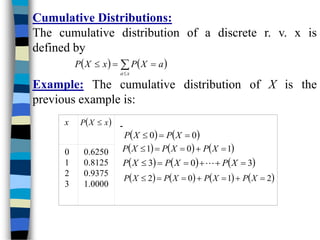
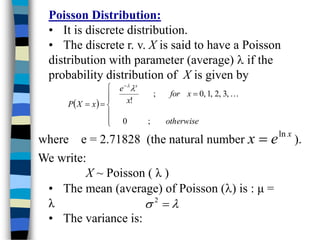
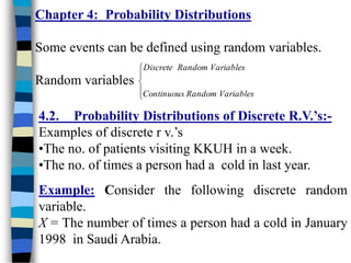
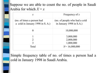
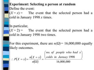
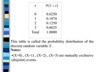
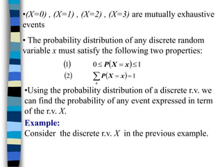
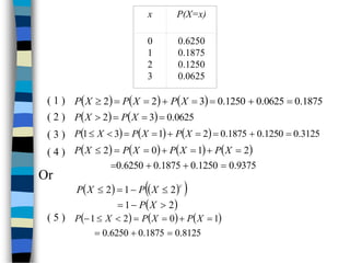
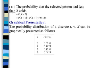
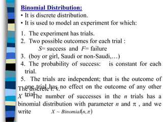
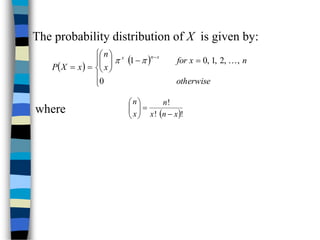
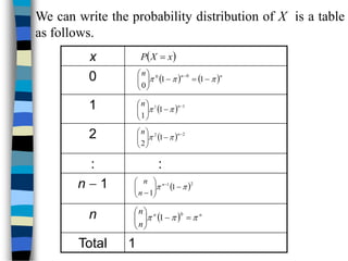
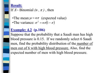
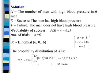
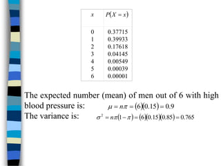
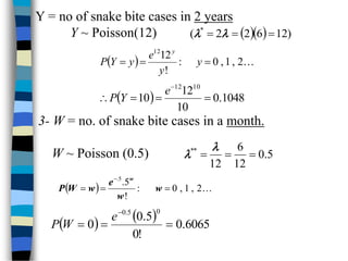
1. The chapter discusses probability distributions of discrete random variables and provides examples. 2. A binomial distribution models experiments with a fixed number of trials, two possible outcomes per trial (success/failure), and a constant probability of success for each trial. 3. For a binomial random variable X with n trials and probability of success π, the mean is nπ and the variance is nπ(1-π).

1. Chapter 4:
Probability Distributions

2. Chapter 4: Probability Distributions
Some events can be defined using random variables.
Random variables





Variables
Random
Continuous
Variables
Random
Discrete
4.2. Probability Distributions of Discrete R.V.’s:-
Examples of discrete r v.’s
•The no. of patients visiting KKUH in a week.
•The no. of times a person had a cold in last year.
Example: Consider the following discrete random
variable.
X = The number of times a person had a cold in January
1998 in Saudi Arabia.

3. Suppose we are able to count the no. of people in Saudi
Arabia for which X = x
x Frequency of x
(no. of times a person had
a cold in January 1998 in S. A.)
(no. of people who had a cold
in January 1998 in S.A.)
0 10,000,000
1
2
3
3,000,000
2,000,000
1,000,000
Total N= 16,000,000
Simple frequency table of no. of times a person had a
cold in January 1998 in Saudi Arabia.

4. Experiment: Selecting a person at random
Define the event:
(X = x) = The event that the selected person had a
cold in January 1998 x times.
In particular,
(X = 2) = The event that the selected person had a
cold in January 1998 two times.
For this experiment, there are n(Ω)= 16,000,000 equally
likely outcomes.
   
  000
,
000
,
16
1998
.














Januay
in
colds
x
had
who
people
of
no
n
x
X
n
x
X
P

5.  
x
X
P 
  1600000
/
x
X
n 

x freq. of x
n(X=x)
0
1
2
3
10000000
3000000
2000000
1000000
0.6250
0.1875
0.1250
0.0625
Total 16000000 1.0000
Note:
   
16000000
Re
16000000
frequency
Frequency
lative
x
X
n
x
X
P






6.  
x
X
P 
x
0
1
2
3
0.6250
0.1874
0.1250
0.0625
Total 1.0000
This table is called the probability distribution of the
discrete random variable X .
Notes:
•(X=0) , (X=1) , (X=2) , (X=3) are mutually exclusive
(disjoint) events.

7. •(X=0) , (X=1) , (X=2) , (X=3) are mutually exhaustive
events
• The probability distribution of any discrete random
variable x must satisfy the following two properties:
    1
0
1 

 x
X
P
    1
2 

 x
X
P
x
•Using the probability distribution of a discrete r.v. we
can find the probability of any event expressed in term
of the r.v. X.
Example:
Consider the discrete r.v. X in the previous example.

8. x P(X=x)
0
1
2
3
0.6250
0.1875
0.1250
0.0625
      1875
.
0
0625
.
0
1250
.
0
3
2
2 






 X
P
X
P
X
P
    0625
.
0
3
2 


 X
P
X
P
      3125
.
0
1250
.
0
1875
.
0
2
1
3
1 







 X
P
X
P
X
P
       
9375
.
0
1250
.
0
1875
.
0
6250
.
0
2
1
0
2










 X
P
X
P
X
P
X
P
( 1 )
( 2 )
( 3 )
( 4 )
Or
   
 
 
2
1
2
1
2







X
P
X
P
X
P
c
     
8125
.
0
1875
.
0
6250
.
0
1
0
2
1









 X
P
X
P
X
P
( 5 )

9.      
8125
.
0
1875
.
0
6250
.
0
1
0
3
.
1
5
.
1









 X
P
X
P
X
P
( 6 )
    0
5
.
3 

 
P
X
P
( 7 )
( 8 ) The probability that the selected person had at least
2 colds
 
    1875
.
0
3
2
2







X
P
X
P
X
P
( 9 ) The probability that the selected person had at most
2 colds
 
9375
.
0
2


 X
P
( 10 ) The probability that the selected person had more
than 2 colds
 
  0625
.
0
3
2





X
P
X
P

10. ( 11 ) The probability that the selected person had less
than 2 colds
 
    8125
.
0
1
0
2







X
P
X
P
X
P
Graphical Presentation:
The probability distribution of a discrete r. v. X can be
graphically presented as follows
x P(X=x)
0
1
2
3
0.6250
0.1875
0.1250
0.0625

11. Population Mean of a Discrete Random
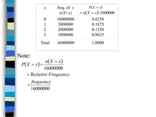
The mean of a discrete random variable X is denoted by
µ and defined by:
 
 

x
x
X
P
x
 [mean = expected value]
Example: We wish to calculate the mean µ of the
discrete r. v. X in the previous example.
 
 
 00
.
1
x
X
P
 
625
.
0


  x
X
xP

x P(X=x) xP(X=x)
0
1
2
3
0.6250
0.1875
0.1250
0.0625
0.0
0.1875
0.2500
0.1875
Total
              625
.
0
0625
.
0
3
125
.
0
2
1875
.
0
1
625
.
0
0 





 
x
x
X
xP


12. Cumulative Distributions:
The cumulative distribution of a discrete r. v. x is
defined by
   





x
a
a
X
P
x
X
P
Example: The cumulative distribution of X is the
previous example is:
 
x
X
P 
   
0
0 

 X
P
X
P
     
1
0
1 



 X
P
X
P
X
P
       
2
1
0
2 





 X
P
X
P
X
P
X
P
     
3
0
3 




 X
P
X
P
X
P 
x
0
1
2
3
0.6250
0.8125
0.9375
1.0000

13. Binomial Distribution:
• It is discrete distribution.
• It is used to model an experiment for which:
1. The experiment has trials.
2. Two possible outcomes for each trial :
S= success and F= failure
3. (boy or girl, Saudi or non-Saudi,…)
4. The probability of success: is constant for each
trial.
5. The trials are independent; that is the outcome of
one trial has no effect on the outcome of any other
trial
The discrete r. v.
X = The number of successes in the n trials has a
binomial distribution with parameter n and  , and we
write  

,
~ n
Binomial
X

14. The probability distribution of X is given by:
 
 


















otherwise
n
x
for
x
n
x
X
P
x
n
x
0
,
,
2
,
1
,
0
1 


 !
!
!
x
n
x
n
x
n










where

15.  
x
X
P 
   n
n
n


 









 
1
1
0
0
0
  1
1
1
1









 n
n


  2
2
1
2









 n
n


 2
1
1
1

 










n
n
n
  n
n
n
n


 








 0
1
We can write the probability distribution of X is a table
as follows.
x
0
1
2
: :
n  1
n
Total 1

16. Result:
If X~ Binomial (n , π ) , then
•The mean: (expected value)
•The variance:

 n

 


 
 1
2
n
Example: 4.2 (p.106)
Suppose that the probability that a Saudi man has high
blood pressure is 0.15. If we randomly select 6 Saudi
men, find the probability distribution of the number of
men out of 6 with high blood pressure. Also, find the
expected number of men with high blood pressure.

17. Solution:
X = The number of men with high blood pressure in 6
men.
S = Success: The man has high blood pressure
F = failure: The man does not have high blood pressure.
•Probability of success P(S) = π = 0.15
•no. of trials n=6
X ~ Binomial (6, 0.16)














6
85
.
0
1
15
.
0
n


The probability distribution of X is:
     

















otherwise
x
x
x
X
P
x
x
;
0
6
,
5
,
4
,
3
,
2
,
1
,
0
;
85
.
0
15
.
0
6 6

18.            37715
.
0
85
.
0
15
.
0
1
85
.
0
15
.
0
0
6
0
6
0
6
0












X
P
          39933
.
0
85
.
0
151
.
0
6
85
.
0
15
.
0
1
6
1
5
5
1












X
P
           17618
.
0
85
.
0
15
.
0
15
85
.
0
15
.
0
2
6
2
4
2
4
2












X
P
           04145
.
0
85
.
0
15
.
0
20
85
.
0
15
.
0
3
6
3
3
3
3
3












X
P
           00549
.
0
85
.
0
15
.
0
15
85
.
0
15
.
0
4
6
4
2
4
2
4












X
P
           00039
.
0
85
.
0
15
.
0
6
85
.
0
15
.
0
5
6
5
1
5
1
5












X
P
           00001
.
0
1
15
.
0
1
85
.
0
15
.
0
6
6
6
0
6
0
6












X
P

19.  
x
X
P 
x
0
1
2
3
4
5
6
0.37715
0.39933
0.17618
0.04145
0.00549
0.00039
0.00001
The expected number (mean) of men out of 6 with high
blood pressure is:
The variance is:
   9
.
0
15
.
0
6 

 
 n
      765
.
0
85
.
0
15
.
0
6
1
2



 

 n

20. Poisson Distribution:
• It is discrete distribution.
• The discrete r. v. X is said to have a Poisson
distribution with parameter (average)  if the
probability distribution of X is given by
 











otherwise
x
for
x
e
x
X
P
x
;
0
,
3
,
2
,
1
,
0
;
!



where e = 2.71828 (the natural number ).
x
e
x ln

We write:
X ~ Poisson ( λ )
• The mean (average) of Poisson () is : μ =
λ
• The variance is:

 
2

21. •The Poisson distribution is used to model a discrete r.
v. which is a count of how many times a specified
random event occurred in an interval of time or space.
Example:
•No. of patients in a waiting room in an hours.
•No. of serious injuries in a particular factory in a
month.
•No. of calls received by a telephone operator in a day.
•No. of rates in each house in a particular city.
Note:
is the average (mean) of the distribution.
If X = The number of calls received in a month and
X ~ Poisson ()

22. then:
(i) Y = The no. calls received in a year.
Y ~ Poisson (*), where *=12
Y ~ Poisson (12)
(ii)W = The no. calls received in a day.
W ~ Poisson (*), where *=/30
W ~ Poisson (/30)
Example:
Suppose that the number of snake bites cases seen at
KKUH in a year has a Poisson distribution with average
6 bite cases.
1- What is the probability that in a year:
(i) The no. of snake bite cases will be 7?
(ii) The no. of snake bite cases will be less than 2?

23. 2- What is the probability that in 2 years there will be 10
bite cases?
3- What is the probability that in a month there will be
no snake bite cases?
Solution:
(1) X = no. of snake bite cases in a year.
X ~ Poisson (6) (=6)
  
,
2
,
1
,
0
;
!
6
6




x
x
e
x
X
P
x
  13768
.
0
!
7
6
)
7
7
6




e
X
P
     
01735
.
0
!
1
6
!
0
6
1
0
2
1
6
0
6










e
e
X
P
X
P
X
P
(i)
(ii)

24. Y = no of snake bite cases in 2 years
Y ~ Poisson(12)    )
12
6
2
2
( *


 

  
2
,
1
,
0
:
!
12
12


 y
y
e
y
Y
P
y
  1048
.
0
10
12
10
10
12





e
Y
P
3- W = no. of snake bite cases in a month.
W ~ Poisson (0.5) 5
.
0
12
6
12
*
*





  
2
,
1
,
0
:
!
5
.
5
.




w
w
e
w
W
P
w
    6065
.
0
!
0
5
.
0
0
0
5
.
0




e
W
P