
![52 2 Vibration Dynamics
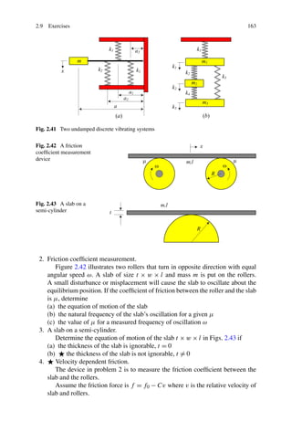
Employing the momentum pi = mi vi of the mass mi , the Newton equation provides
us with the equation of motion of the system:
d d
Fi = pi = (mi vi ) (2.1)
dt dt
When the motion of a massive body with mass moment Ii is rotational, then its equa-
tion of motion will be found by Euler equation, in which we employ the moment of
momentum Li = Ii ω of the mass mi :
d d
Mi = Li = (Ii ω) (2.2)
dt dt
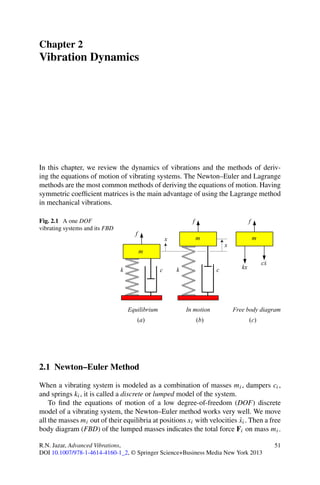
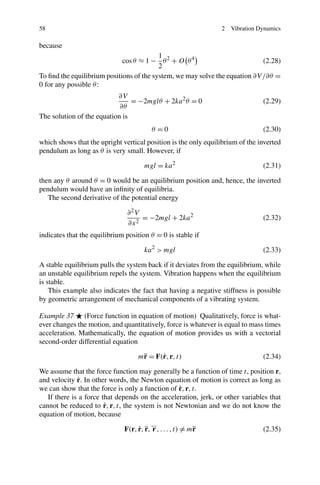
For example, Fig. 2.1 illustrates a one degree-of-freedom (DOF) vibrating sys-
tem. Figure 2.1(b) depicts the system when m is out of the equilibrium position at x
˙
and moving with velocity x, both in positive direction. The FBD of the system is as
shown in Fig. 2.1(c). The Newton equation generates the equations of motion:
ma = −cv − kx + f (x, v, t) (2.3)
The equilibrium position of a vibrating system is where the potential energy of
the system, V , is extremum:
∂V
=0 (2.4)
∂x
We usually set V = 0 at the equilibrium position. Linear systems with constant
stiffness have only one equilibrium or infinity equilibria, while nonlinear systems
may have multiple equilibria. An equilibrium is stable if
∂ 2V
>0 (2.5)
∂x 2
and is unstable if
∂ 2V
<0 (2.6)
∂x 2
The geometric arrangement and the number of employed mechanical elements
can be used to classify discrete vibrating systems. The number of masses times the
DOF of each mass makes the total DOF of the vibrating system n. Each indepen-
dent DOF of a mass is indicated by an independent variable, called the generalized
coordinate. The final set of equations would be n second-order differential equa-
tions to be solved for n generalized coordinates. When each moving mass has one
DOF, then the system’s DOF is equal to the number of masses. The DOF may
also be defined as the minimum number of independent coordinates that defines the
configuration of a system.
The equation of motion of an n DOF linear mechanical vibrating system of can
always be arranged as a set of second-order differential equations
[m]¨ + [c]˙ + [k]x = F
x x (2.7)](https://image.slidesharecdn.com/advancedvibrations-130411024927-phpapp01/85/Advanced-vibrations-2-320.jpg)
![2.1 Newton–Euler Method 53
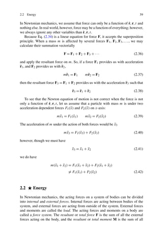
Fig. 2.2 Two, three, and one
DOF models for vertical
vibrations of vehicles
Fig. 2.3 A 1/8 car model
and its free body diagram
in which, x is a column array of describing coordinates of the system, and f is a
column array of the associated applied forces. The square matrices [m], [c], [k] are
the mass, damping, and stiffness matrices.
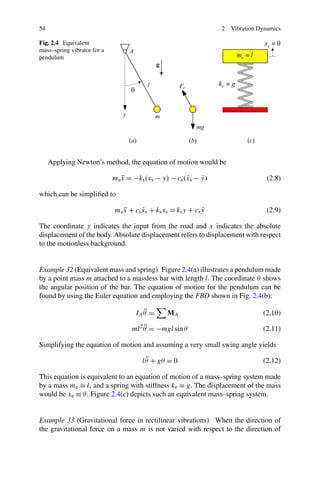
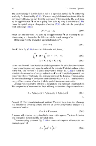
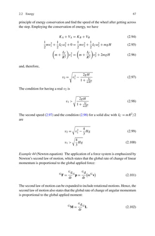
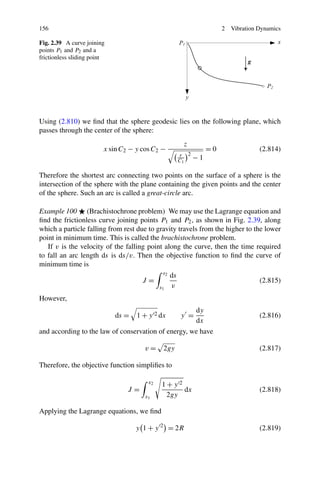
Example 30 (The one, two, and three DOF model of vehicles) The one, two, and
three DOF model for analysis of vertical vibrations of a vehicle are shown in
Fig. 2.2(a)–(c). The system in Fig. 2.2(a) is called the quarter car model, in which
ms represents a quarter mass of the body, and mu represents a wheel. The param-
eters ku and cu are models for tire stiffness and damping. Similarly, ks and cu are
models for the main suspension of the vehicle. Figure 2.2(c) is called the 1/8 car
model, which does not show the wheel of the car, and Fig. 2.2(b) is a quarter car
with a driver md . The driver’s seat is modeled by kd and cd .
Example 31 (1/8 car model) Figure 2.3(a) shows the simplest model for vertical
vibrations of a vehicle. This model is sometimes called 1/8 car model. The mass ms
represents one quarter of the car’s body, which is mounted on a suspension made of
a spring ks and a damper cs . When ms is at a position such as shown in Fig. 2.3(b),
its free body diagram is as in Fig. 2.3(c).](https://image.slidesharecdn.com/advancedvibrations-130411024927-phpapp01/85/Advanced-vibrations-3-320.jpg)
![56 2 Vibration Dynamics
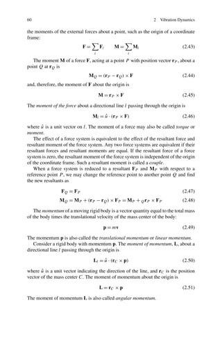
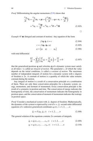
Fig. 2.6 A 1/4 car model
and its free body diagram
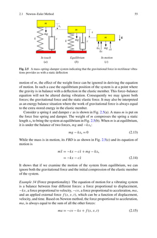
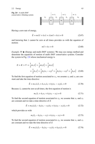
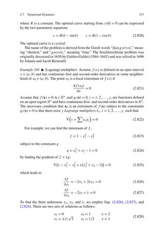
Example 35 (A two DOF base excited system) Figure 2.6(a)–(c) illustrate the equi-
librium, motion, and FBD of a two DOF system. The FBD is plotted based on the
assumption
xs > x u > y (2.16)
Applying Newton’s method provides us with two equations of motion:
ms xs = −ks (xs − xu ) − cs (xs − xu )
¨ ˙ ˙ (2.17)
mu xu = ks (xs − xu ) + cs (xs − xu )
¨ ˙ ˙
− ku (xu − y) − cu (xu − y)
˙ ˙ (2.18)
The assumption (2.16) is not necessary. We can find the same Eqs. (2.17)
and (2.18) using any other assumption, such as xs < xu > y, xs > xu < y, or
xs < xu < y. However, having an assumption helps to make a consistent free body
diagram.
We usually arrange the equations of motion for a linear system in a matrix form
to take advantage of matrix calculus:
[M]˙ + [C]˙ + [K]x = F
x x (2.19)
Rearrangement of Eqs. (2.17) and (2.18) yields
ms 0 ¨
xs cs −cs ˙
xs
+
0 mu ¨
xu −cs cs + cu ˙
xu
ks −ks xs 0
+ = (2.20)
−ks ks + ku xu ku y + c u y
˙
Example 36 (Inverted pendulum and negative stiffness) Figure 2.7(a) illustrates
an inverted pendulum with a tip mass m and a length l. The pendulum is supported](https://image.slidesharecdn.com/advancedvibrations-130411024927-phpapp01/85/Advanced-vibrations-6-320.jpg)
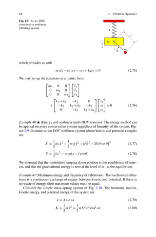
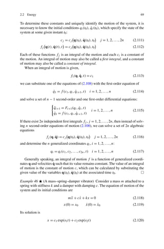
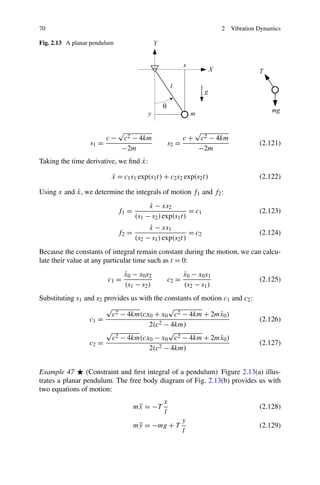
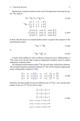
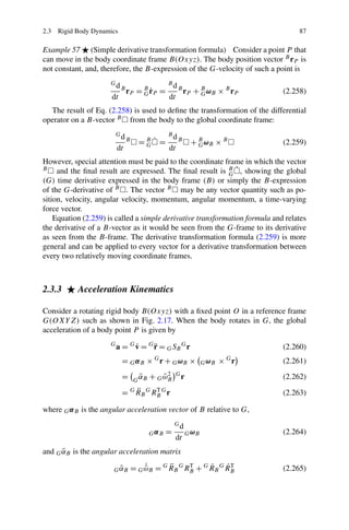
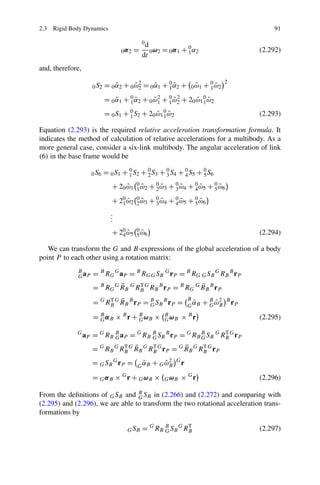
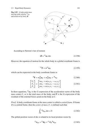
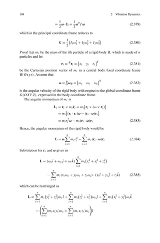
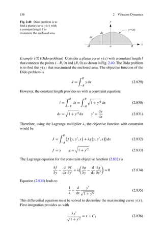
![2.3 Rigid Body Dynamics 73
Fig. 2.14 A globally fixed
G-frame and a body B-frame
with a fixed common origin
at O
2.3 Rigid Body Dynamics
A rigid body may have three translational and three rotational DOF. The transla-
tional and rotational equations of motion of the rigid body are determined by the
Newton–Euler equations.
2.3.1 Coordinate Frame Transformation
Consider a rotation of a body coordinate frame B(Oxyz) with respect to a global
frame G(OXY Z) about their common origin O as illustrated in Fig. 2.14. The com-
ponents of any vector r may be expressed in either frame. There is always a trans-
formation matrix G RB to map the components of r from the frame B(Oxyz) to the
other frame G(OXY Z):
G
r = G RB B r (2.151)
−1
In addition, the inverse map B r = G RB G r can be done by B RG ,
B
r = B RG G r (2.152)
where
G B
RB = RG = 1 (2.153)
and
−1
B
RG = G RB = G RB
T
(2.154)
When the coordinate frames B and G are orthogonal, the rotation matrix GR
B is
called an orthogonal matrix. The transpose R T and inverse R −1 of an orthogonal
matrix [R] are equal:
R T = R −1 (2.155)](https://image.slidesharecdn.com/advancedvibrations-130411024927-phpapp01/85/Advanced-vibrations-23-320.jpg)
![78 2 Vibration Dynamics
B
r = Ry,−45 Rx,−45 G r
⎡ ⎤ ⎡1 ⎤⎡ ⎤
cos −π 0 − sin −π 0 0 1
⎦ ⎢0 cos 4 sin −π ⎥ ⎣2⎦
4 4 −π
=⎣ 0 1 0 ⎣ 4 ⎦
sin −π 0 cos −π
4 4 0 − sin −π cos −π 3
4 4
⎡ ⎤⎡ ⎤ ⎡ ⎤
0.707 0.5 0.5 1 3.207
=⎣ 0 0.707 −0.707⎦ ⎣2⎦ = ⎣−0.707⎦ (2.185)
−0.707 0.5 0.5 3 1.793
To check this result, let us change the role of B and G. So, the body point at
⎡ ⎤
1
B
r = ⎣2⎦ (2.186)
3
undergoes an active rotation of 45 deg about the x-axis followed by 45 deg about
the y-axis. The global coordinates of the point would be
B
r = Ry,45 Rx,45 G r (2.187)
so
G
r = [Ry,45 Rx,45 ]TB r = Rx,45 Ry,45 B r
T T
(2.188)
Example 52 (Multiple rotations about body axes) Consider a globally fixed point P
at
⎡ ⎤
1
G
r = ⎣2⎦ (2.189)
3
The body B will turn 45 deg about the x-axis and then 45 deg about the y-axis.
An observer in B will see P at
B
r = RY,−45 RX,−45 G r
⎡ ⎤ ⎡1 ⎤⎡ ⎤
cos −π 0 sin −π 0 0 1
4 4 ⎢ −π −π ⎥
=⎣ 0 1 0 ⎦ ⎣0 cos 4 − sin 4 ⎦ ⎣2⎦
− sin −π 0 cos −π
4 4 0 sin −π cos −π 3
4 4
⎡ ⎤⎡ ⎤ ⎡ ⎤
0.707 0.5 −0.5 1 0.20711
=⎣ 0 0.707 0.707⎦ ⎣2⎦ = ⎣ 3.5356 ⎦ (2.190)
0.707 −0.5 0.5 3 1.2071
Example 53 (Successive rotations about global axes) After a series of sequential
rotations R1 , R2 , R3 , . . . , Rn about the global axes, the final global position of a
body point P can be found by
G
r = G RB B r (2.191)](https://image.slidesharecdn.com/advancedvibrations-130411024927-phpapp01/85/Advanced-vibrations-28-320.jpg)
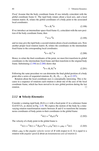
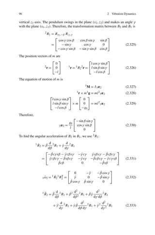
![2.3 Rigid Body Dynamics 83
˜
We denote the coefficient of G r(t) by G ωB
˜
G ωB ˙
= G R B G RB
T
(2.221)
and rewrite Eq. (2.220) as
G
v = G ωB G r(t)
˜ (2.222)
or equivalently as
G
v = G ωB × G r(t) (2.223)
where G ωB is the instantaneous angular velocity of the body B relative to the global
frame G as seen from the G-frame.
Transforming G v to the body frame provides us with the body expression of the
velocity vector:
T ˙
B
G vP = G RB G v = G RB G ω B G r = G RB G R B G RB G r
T T
˜ T
T ˙
= G RB G R B B r (2.224)
G˜
We denote the coefficient of B r by B ωB
T ˙
B
˜
G ωB = G RB G R B (2.225)
and rewrite Eq. (2.224) as
B
G vP = B ω B B rP
G˜ (2.226)
or equivalently as
B
G vP = B ω B × B rP
G (2.227)
where Bω is the instantaneous angular velocity of B relative to the global frame
G B
G as seen from the B-frame.
The time derivative of the orthogonality condition, G RB G RB = I, introduces an
T
important identity,
G ˙ T ˙T
R B G RB + G RB G R B = 0 (2.228)
˜ ˙
which can be used to show that the angular velocity matrix G ωB = [G RB G RB ] is
T
skew-symmetric:
G ˙T
RB G R B =
G ˙ T
R B G RB
T
(2.229)
Generally speaking, an angular velocity vector is the instantaneous rotation of
a coordinate frame A with respect to another frame B that can be expressed in or
seen from a third coordinate frame C. We indicate the first coordinate frame A by
a right subscript, the second frame B by a left subscript, and the third frame C by
a left superscript, C ωA . If the left super and subscripts are the same, we only show
B
the subscript.](https://image.slidesharecdn.com/advancedvibrations-130411024927-phpapp01/85/Advanced-vibrations-33-320.jpg)
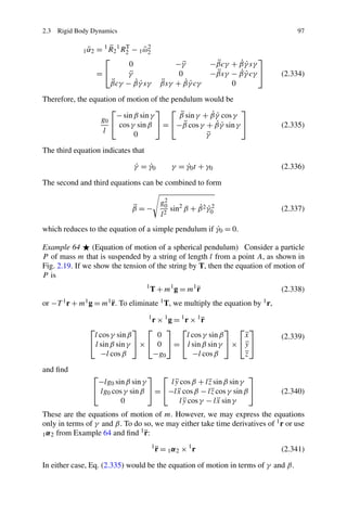
![2.3 Rigid Body Dynamics 85
Substituting the derivative of the rotation matrices with
0 ˙
R 2 = 0 ω 2 0 R2
˜ (2.242)
0 ˙
R 1 = 0 ω 1 R1
˜ 0
(2.243)
1 ˙
R 2 = 1 ω 2 1 R2
˜ (2.244)
results in
˜
0 ω2
0
R2 = 0 ω1 0 R1 1 R2 + 0 R11 ω2 1 R2
˜ ˜
= 0 ω1 0 R2 + 0 R11 ω2 0 R1 0 R1 1 R2
˜ ˜ T
= 0 ω 1 0 R2 + 0 ω 2 0 R2
˜ 1˜ (2.245)
where
0
R11 ω2 0 R1 = 0 ω2
˜ T
1˜ (2.246)
Therefore, we find
˜
0 ω2 = 0 ω1 + 0 ω2
˜ 1˜ (2.247)
which indicates that two angular velocities may be added when they are expressed
in the same frame:
0 ω2 = 0 ω1 + 0 ω2
1 (2.248)
The expansion of this equation for any number of angular velocities would be
Eq. (2.214).
Employing the relative angular velocity formula (2.248), we can find the relative
velocity formula of a point P in B2 at 0 rP :
0 v2 = 0 ω 2 0 rP = 0 ω1 + 0 ω 2 0 rP = 0 ω 1 0 rP + 0 ω 2 0 rP
1 1
= 0 v1 + 0 v2
1 (2.249)
˜ G˜
The angular velocity matrices G ωB and B ωB are skew-symmetric and not invert-
ible. However, we can define their inverse by the rules
˜ −1
G ωB ˙ −1
= G RB G R B (2.250)
B −1
˜
G ωB
˙ −1
= G R B G RB (2.251)
to get
˜ −1 ˜
G ωB G ωB ˜ ˜ −1
= G ωB G ωB = [I] (2.252)
B −1 B
˜ ˜
G ωB G ωB = B
˜ B ˜ −1
G ωB G ωB = [I] (2.253)](https://image.slidesharecdn.com/advancedvibrations-130411024927-phpapp01/85/Advanced-vibrations-35-320.jpg)
![86 2 Vibration Dynamics
Example 55 (Rotation of a body point about a global axis) Consider a rigid body
is turning about the Z-axis with a constant angular speed α = 10 deg/s. The global
˙
velocity of a body point at P (5, 30, 10) when the body is at α = 30 deg is
G ˙
vP = G RB (t)B rP
⎛⎡ ⎤⎞ ⎡ ⎤
Gd cos α − sin α 0 5
= ⎝⎣ sin α cos α 0⎦⎠ ⎣30⎦
dt 0 0 1 10
⎡ ⎤⎡ ⎤
− sin α − cos α 0 5
= α ⎣ cos α − sin α 0⎦ ⎣30⎦
˙
0 0 0 10
⎡ ⎤⎡ ⎤ ⎡ ⎤
− sin π − cos π 0 5 −4.97
10π ⎣ 6 6
= cos π
6 − sin π 0⎦ ⎣30⎦ = ⎣−1.86⎦
6 (2.254)
180 0 0 0 10 0
The point P is now at
G
r P = G RB B r P
⎡ ⎤⎡ ⎤ ⎡ ⎤
cos π − sin π
6 6 0 5 −10.67
= ⎣ sin π cos π 0⎦ ⎣30⎦ = ⎣ 28.48 ⎦ (2.255)
6 6
0 0 1 10 10
Example 56 (Rotation of a global point about a global axis) A body point P at
Br
P = [5 30 10]T is turned α = 30 deg about the Z-axis. The global position of P
is at
G
r P = G RB B r P
⎡ ⎤⎡ ⎤ ⎡ ⎤
cos π − sin π
6 6 0 5 −10.67
= ⎣ sin π cos π 0⎦ ⎣30⎦ = ⎣ 28.48 ⎦ (2.256)
6 6
0 0 1 10 10
If the body is turning with a constant angular speed α = 10 deg/s, the global velocity
˙
of the point P would be
G ˙
v P = G R B G RB G r P
T
⎡ π ⎤⎡ π ⎤T ⎡ ⎤
−s −c π 0 c6 −s π 0 −10.67
10π ⎣ π6 6 6
= c6 −s π
6 0⎦ ⎣ s π
6 cπ6 0⎦ ⎣ 28.48 ⎦
180 0 0 0 0 0 1 10
⎡ ⎤
−4.97
= ⎣−1.86⎦ (2.257)
0](https://image.slidesharecdn.com/advancedvibrations-130411024927-phpapp01/85/Advanced-vibrations-36-320.jpg)
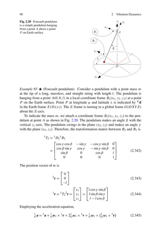
![2.3 Rigid Body Dynamics 93
Example 59 (Rotation of a global point about a global axis) A body point P at
B r = [5 30 10]T cm is turning with a constant angular acceleration α = 2 rad/s2
¨
P
about the Z-axis. When the body frame is at α = 30 deg, its angular speed
α = 10 deg/s.
˙
The transformation matrix G RB between the B- and G-frames is
⎡ ⎤ ⎡ ⎤
cos π − sin π 0
6 6 0.866 −0.5 0
G
RB = ⎣ sin π
6 cos π6 0⎦ ≈ ⎣ 0.5 0.866 0⎦ (2.307)
0 0 1 0 0 1
and, therefore, the acceleration of point P is
⎡ ⎤
1010
G ¨
aP = G RB G RB G rP = ⎣−2869.4⎦ cm/s2
T
(2.308)
0
where
G d2 Gd G d2
G
RB = α
¨ G
RB − α 2
˙ G
RB (2.309)
dt 2 dα dα 2
is the same as (2.305).
Example 60 (B-expression of angular acceleration) The angular acceleration ex-
pressed in the body frame is the body derivative of the angular velocity vector. To
show this, we use the derivative transport formula (2.259):
Gd
G˙
= B ωB =
B B
GαB G ωB
dt
Bd Bd
= B
G ωB + B ωB × B ωB =
G G
B
G ωB (2.310)
dt dt
Interestingly, the global and body derivatives of B ωB are equal:
G
Gd Bd
B
G ωB = B
G ωB = B αB
G (2.311)
dt dt
ˆ
This is because G ωB is about an axis u that is instantaneously fixed in both B and G.
A vector α can generally indicate the angular acceleration of a coordinate frame
A with respect to another frame B. It can be expressed in or seen from a third
coordinate frame C. We indicate the first coordinate frame A by a right subscript,
the second frame B by a left subscript, and the third frame C by a left superscript,
C α . If the left super and subscripts are the same, we only show the subscript. So,
B A
the angular acceleration of A with respect to B as seen from C is the C-expression
of B αA :
C
B αA = C RB B αA (2.312)](https://image.slidesharecdn.com/advancedvibrations-130411024927-phpapp01/85/Advanced-vibrations-43-320.jpg)
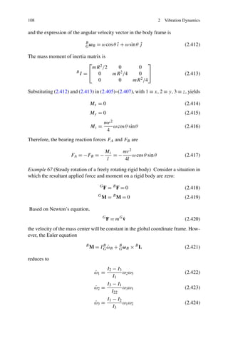
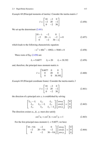
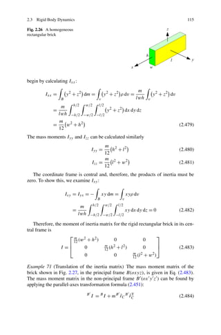
![110 2 Vibration Dynamics
where δij is Kronecker’s delta (2.171),
1 if m = n
δmn = (2.434)
0 if m = n
The elements of I are calculated in a body coordinate frame attached to the mass
center C of the body. Therefore, I is a frame-dependent quantity and must be written
with a frame indicator such as B I to show the frame in which it is computed:
⎡ 2 ⎤
y + z2 −xy −zx
B
I= ⎣ −xy z2 + x 2 −yz ⎦ dm (2.435)
B −zx −yz x 2 + y2
= r 2 I − r rT dm = −˜ r dm
r˜ (2.436)
B B
˜
where r is the associated skew-symmetric matrix of r:
⎡ ⎤
0 −r3 r2
r = ⎣ r3
˜ 0 −r1 ⎦ (2.437)
−r2 r1 0
The moments of inertia can be transformed from a coordinate frame B1 to an-
other coordinate frame B2 , both defined at the mass center of the body, according to
the rule of the rotated-axes theorem:
B2
I = B2 RB1 B1 I B2 RB1
T
(2.438)
Transformation of the moment of inertia from a central frame B1 located at B2 rC to
another frame B2 , which is parallel to B1 , is, according to the rule of the parallel-
axes theorem:
B2
I = B1 I + m rC rC
˜ ˜T (2.439)
If the local coordinate frame Oxyz is located such that the products of inertia
vanish, the local coordinate frame is the principal coordinate frame and the associ-
ated mass moments are principal mass moments. Principal axes and principal mass
moments can be found by solving the following characteristic equation for I :
Ixx − I Ixy Ixz
Iyx Iyy − I Iyz = 0 (2.440)
Izx Izy Izz − I
det [Iij ] − I [δij ] = 0 (2.441)
Equation (2.441) is a cubic equation in I , so we obtain three eigenvalues,
I1 = Ix I2 = Iy I3 = Iz (2.442)](https://image.slidesharecdn.com/advancedvibrations-130411024927-phpapp01/85/Advanced-vibrations-60-320.jpg)
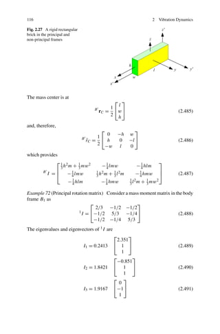
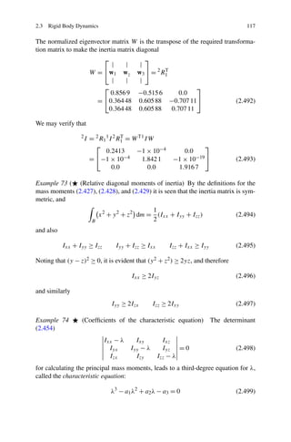
![118 2 Vibration Dynamics
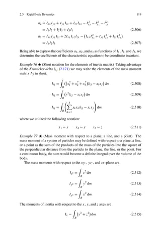
The coefficients of the characteristic equation are called the principal invariants
of [I ]. The coefficients of the characteristic equation can directly be found from
a1 = Ixx + Iyy + Izz = tr [I ] (2.500)
a2 = Ixx Iyy + Iyy Izz + Izz Ixx − Ixy − Iyz − Izx
2 2 2
Ixx Ixy I Iyz I Ixz
= + yy + xx
Iyx Iyy Izy Izz Izx Izz
1 2
= a − tr I 2 (2.501)
2 1
a3 = Ixx Iyy Izz + Ixy Iyz Izx + Izy Iyx Ixz
− (Ixx Iyz Izy + Iyy Izx Ixz + Izz Ixy Iyx )
= Ixx Iyy Izz + 2Ixy Iyz Izx − Ixx Iyz + Iyy Izx + Izz Ixy
2 2 2
= det [I ] (2.502)
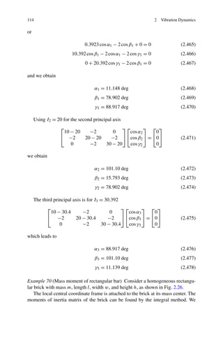
Example 75 (The principal mass moments are coordinate invariants) The roots
of the inertia characteristic equation are the principal mass moments. They are all
real but not necessarily different. The principal mass moments are extreme. That
is, the principal mass moments determine the smallest and the largest values of Iii .
Since the smallest and largest values of Iii do not depend on the choice of the body
coordinate frame, the solution of the characteristic equation is not dependent of the
coordinate frame.
In other words, if I1 , I2 , and I3 are the principal mass moments for B1 I , the
principal mass moments for B2 I are also I1 , I2 , and I3 when
B2
I = B2 RB1 B1 I B2 RB1
T
We conclude that I1 , I2 , and I3 are coordinate invariants of the matrix [I ], and
therefore any quantity that depends on I1 , I2 , and I3 is also coordinate invariant.
Because the mass matrix [I ] has rank 3, it has only three independent invariants and
every other invariant can be expressed in terms of I1 , I2 , and I3 .
Since I1 , I2 , and I3 are the solutions of the characteristic equation of [I ] given in
(2.499), we may write the determinant (2.454) in the form
(λ − I1 )(λ − I2 )(λ − I3 ) = 0 (2.503)
The expanded form of this equation is
λ3 − (I1 + I2 + I3 )λ2 + (I1 I2 + I2 I3 + I3 I1 )a2 λ − I1 I2 I3 = 0 (2.504)
By comparing (2.504) and (2.499) we conclude that
a1 = Ixx + Iyy + Izz = I1 + I2 + I3 (2.505)](https://image.slidesharecdn.com/advancedvibrations-130411024927-phpapp01/85/Advanced-vibrations-68-320.jpg)
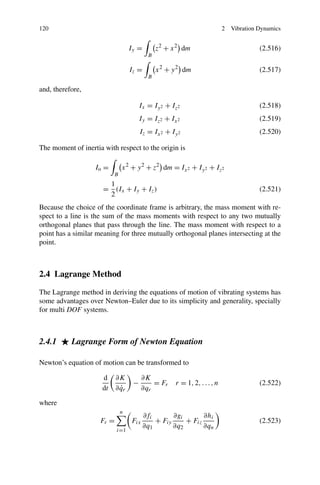
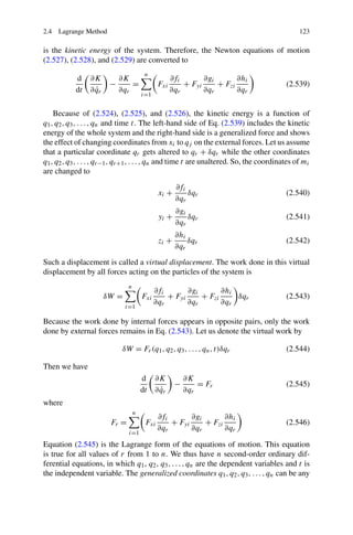
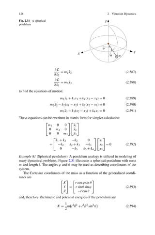
![2.4 Lagrange Method 121
Equation (2.522) is called the Lagrange equation of motion, where K is the kinetic
energy of the n DOF system, qr , r = 1, 2, . . . , n are the generalized coordinates of
the system, Fi = [Fix Fiy Fiz ]T is the external force acting on the ith particle of the
system, and Fr is the generalized force associated to qr . The functions fi , gi , hi ,
are the relationships of x1 , yi , zi , based on the generalized coordinates of the system
xi = fi (qj , t), yi = gi (qj , t), zi = hi (qj , t).
Proof Let mi be the mass of one of the particles of a system and let (xi , yi , zi )
be its Cartesian coordinates in a globally fixed coordinate frame. Assume that the
coordinates of every individual particle are functions of another set of coordinates
q1 , q2 , q3 , . . . , qn , and possibly time t:
xi = fi (q1 , q2 , q3 , . . . , qn , t) (2.524)
yi = gi (q1 , q2 , q3 , . . . , qn , t) (2.525)
zi = hi (q1 , q2 , q3 , . . . , qn , t) (2.526)
If Fxi , Fyi , Fzi are components of the total force acting on the particle mi , then
the Newton equations of motion for the particle would be
Fxi = mi xi
¨ (2.527)
Fyi = mi yi
¨ (2.528)
Fzi = mi zi
¨ (2.529)
We multiply both sides of these equations by ∂fi /∂qr , ∂gi /∂qr , and ∂hi /∂qr , re-
spectively, and add them up for all the particles to find
n n
∂fi ∂gi ∂hi ∂fi ∂gi ∂hi
mi ¨
xi + yi
¨ + zi
¨ = Fxi + Fyi + Fzi (2.530)
∂qr ∂qr ∂qr ∂qr ∂qr ∂qr
i=1 i=1
where n is the total number of particles.
Taking the time derivative of Eq. (2.524),
∂fi ∂fi ∂fi ∂fi ∂fi
˙
xi = q1 +
˙ q2 +
˙ q3 + · · · +
˙ qn +
˙ (2.531)
∂q1 ∂q2 ∂q3 ∂qn ∂t
we find
˙
∂ xi ∂ ∂fi ∂fi ∂fi ∂fi ∂fi
= q1 +
˙ q2 + · · · +
˙ qn +
˙ = (2.532)
˙
∂ qr ˙
∂ qr ∂q1 ∂q2 ∂qn ∂t ∂qr
and, therefore,
∂fi ˙
∂ xi d ˙
∂ xi d ˙
∂ xi
¨
xi = xi
¨ = ˙
xi − xi
˙ (2.533)
∂qr ˙
∂ qr dt ˙
∂ qr dt ˙
∂ qr](https://image.slidesharecdn.com/advancedvibrations-130411024927-phpapp01/85/Advanced-vibrations-71-320.jpg)
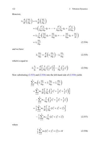
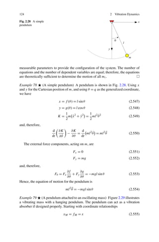
![126 2 Vibration Dynamics
¨ ˙
(M + m)x + ml θ cos θ − ml θ 2 sin θ = −kx
¨ (2.568)
2¨
ml θ + ml x cos θ = −mgl sin θ
¨ (2.569)
2.4.2 Lagrangean Mechanics
Let us assume that for some forces F = [Fix Fiy Fiz ]T there is a function V , called
potential energy, such that the force is derivable from V
F = −∇V (2.570)
Such a force is called a potential or conservative force. Then the Lagrange equation
of motion can be written as
d ∂L ∂L
− = Qr r = 1, 2, . . . , n (2.571)
dt ˙
∂ qr ∂qr
where
L=K −V (2.572)
is the Lagrangean of the system and Qr is the nonpotential generalized force
n
∂fi ∂gi ∂hi
Qr = Fix + Fiy + Fiz (2.573)
∂q1 ∂q2 ∂qn
i=1
for which there is no potential function.
Proof Assume that the external forces F = [Fxi Fyi Fzi ]T acting on the system are
conservative:
F = −∇V (2.574)
The work done by these forces in an arbitrary virtual displacement δq1 , δq2 ,
δq3 , . . . , δqn is
∂V ∂V ∂V
∂W = − δq1 − δq2 − · · · δqn (2.575)
∂q1 ∂q2 ∂qn
and then the Lagrange equation becomes
d ∂K ∂K ∂V
− =− r = 1, 2, . . . , n (2.576)
dt ˙
∂ qr ∂qr ∂q1
Introducing the Lagrangean function L = K − V converts the Lagrange equation of
a conservative system to
d ∂L ∂L
− = 0 r = 1, 2, . . . , n (2.577)
dt ˙
∂ qr ∂qr](https://image.slidesharecdn.com/advancedvibrations-130411024927-phpapp01/85/Advanced-vibrations-76-320.jpg)
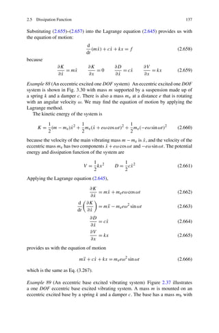
![2.5 Dissipation Function 135
2.5 Dissipation Function
The Lagrange equation,
d ∂K ∂K
− = Fr r = 1, 2, . . . , n (2.643)
dt ˙
∂ qr ∂qr
or
d ∂L ∂L
− = Qr r = 1, 2, . . . , n (2.644)
dt ˙
∂ qr ∂qr
as introduced in Eqs. (2.522) and (2.571) can both be applied to find the equations
of motion of a vibrating system. However, for small and linear vibrations, we may
use a simpler and more practical Lagrange equation, thus:
d ∂K ∂K ∂D ∂V
− + + = fr r = 1, 2, . . . , n (2.645)
dt ˙
∂ qr ∂qr ˙
∂ qr ∂qr
where K is the kinetic energy, V is the potential energy, and D is the dissipation
function of the system
n n
1 1
˙ ˙
K = qT [m]q = ˙ ˙
qi mij qj (2.646)
2 2
i=1 j =1
n n
1 1
V = qT [k]q = qi kij qj (2.647)
2 2
i=1 j =1
n n
1 1
˙ ˙
D = qT [c]q = ˙ ˙
qi cij qj (2.648)
2 2
i=1 j =1
and fr is the applied force on the mass mr .
Proof Consider a one DOF mass–spring–damper vibrating system. When viscous
damping is the only type of damping in the system, we may employ a function
known as the Rayleigh dissipation function
1
D = cx 2
˙ (2.649)
2
to find the damping force fc by differentiation:
∂D
fc = − (2.650)
˙
∂x
Remembering that the elastic force fk can be found from a potential energy V
∂V
fk = − (2.651)
∂x](https://image.slidesharecdn.com/advancedvibrations-130411024927-phpapp01/85/Advanced-vibrations-85-320.jpg)
![140 2 Vibration Dynamics
The virtual work of the dissipation force is
n1
δW = Qi δqi (2.687)
i=1
n1
∂vk
Qi = − ck fk (vk ) (2.688)
˙
∂ qi
k=1
where n1 is the total number of dissipation forces. By introducing the dissipation
function D as
n1 vi
D= ck fk (zk ) dz (2.689)
i=1 0
we have
∂D
Qi = − (2.690)
˙
∂ qi
The dissipation power P of the dissipation force Qi is
n n
∂D
P= Qi qi =
˙ ˙
qi (2.691)
˙
∂ qi
i=1 i=1
2.6 Quadratures
If [m] is an n × n square matrix and x is an n × 1 vector, then S is a scalar function
called quadrature and is defined by
S = xT [m]x (2.692)
The derivative of the quadrature S with respect to the vector x is
∂S
= [m] + [m]T x (2.693)
∂x
Kinetic energy K, potential energy V , and dissipation function D are quadratures
1
˙
K = xT [m]˙x (2.694)
2
1
V = xT [k]x (2.695)
2
1
˙
D = xT [c]˙
x (2.696)
2](https://image.slidesharecdn.com/advancedvibrations-130411024927-phpapp01/85/Advanced-vibrations-90-320.jpg)
![2.6 Quadratures 141
and, therefore,
∂K 1
= [m] + [m]T x ˙ (2.697)
˙
∂x 2
∂V 1
= [k] + [k]T x (2.698)
∂x 2
∂D 1
˙
= [c] + [c]T x (2.699)
˙
∂x 2
Employing quadrature derivatives and the Lagrange method,
d ∂K ∂K ∂D ∂V
+ + + =F (2.700)
˙
dt ∂ x ∂x ˙
∂x ∂x
δW = FT ∂x (2.701)
the equation of motion for a linear n degree-of-freedom vibrating system becomes
[m]¨ + [c]˙ + [k]x = F
x x (2.702)
where [m], [c], [k] are symmetric matrices:
1
[m] = [m] + [m]T (2.703)
2
1
[c] = [c] + [c]T (2.704)
2
1
[k] = [k] + [k]T (2.705)
2
Quadratures are also called Hermitian forms.
Proof Let us define a general asymmetric quadrature as
S = xT [a]y = xi aij yj (2.706)
i j
If the quadrature is symmetric, then x = y and
S = xT [a]x = xi aij xj (2.707)
i j
The vectors x and y may be functions of n generalized coordinates qi and time t:
x = x(q1 , q2 , . . . , qn , t) (2.708)
y = y(q1 , q2 , . . . , qn , t) (2.709)
T
q = q1 q2 · · · qn (2.710)](https://image.slidesharecdn.com/advancedvibrations-130411024927-phpapp01/85/Advanced-vibrations-91-320.jpg)
![142 2 Vibration Dynamics
The derivative of x with respect to q is a square matrix
⎡ ∂x1 ∂x2 ∂xn ⎤
∂q1 ∂q1 ··· ∂q1
⎢ ∂x1 ⎥
∂x ⎢ ∂q ∂x2
··· ...⎥
= ⎢ 2 ∂q2 ⎥ (2.711)
∂q ⎢ . . .
⎣ ··· ...
⎥
···⎦
∂x1 ∂xn
∂qn ··· ··· ∂qn
which can also be expressed by
⎡ ∂x ⎤
∂q1
⎢ ∂x ⎥
∂x ⎢ ∂q ⎥
= ⎢ 2⎥ (2.712)
∂q ⎢ . . . ⎥
⎣ ⎦
∂x
∂qn
or
∂x ∂x1 ∂x2 ∂xn
= ∂q ∂q ... ∂q (2.713)
∂q
The derivative of S with respect to an element of qk is
∂S ∂
= xi aij yj
∂qk ∂qk
i j
∂xi ∂yj
= aij yj + xi aij
∂qk ∂qk
i j i j
∂xi ∂yj
= aij yj + aij xi
∂qk ∂qk
j i i j
∂xi ∂yi
= aij yj + aj i xj (2.714)
∂qk ∂qk
j i j i
and, hence, the derivative of S with respect to q is
∂S ∂x ∂y T
= [a]y + [a] x (2.715)
∂q ∂q ∂q
If S is a symmetric quadrature, then
∂S ∂ T ∂x ∂x T
= x [a]x = [a]x + [a] x (2.716)
∂q ∂q ∂q ∂q](https://image.slidesharecdn.com/advancedvibrations-130411024927-phpapp01/85/Advanced-vibrations-92-320.jpg)
![2.6 Quadratures 143
and if q = x, then the derivative of a symmetric S with respect to x is
∂S ∂ T ∂x ∂x
= x [a]x = [a]x + [a]T x
∂x ∂x ∂x ∂x
= [a]x + [a]T x = [a] + [a]T x (2.717)
If [a] is a symmetric matrix, then
[a] + [a]T = 2[a] (2.718)
however, if [a] is not a symmetric matrix, then [a] = [a] + [a]T is a symmetric
matrix because
a ij = aij + aj i = aj i + aij = a j i (2.719)
and, therefore,
[a] = [a]T (2.720)
Kinetic energy K, potential energy V , and dissipation function D can be ex-
pressed by quadratures:
1
˙
K = xT [m]˙x (2.721)
2
1
V = xT [k]x (2.722)
2
1
˙
D = xT [c]˙
x (2.723)
2
Substituting K, V , and D in the Lagrange equation provides us with the equations
of motion:
d ∂K ∂K ∂D ∂V
F= + + +
˙
dt ∂ x ∂x ˙
∂x ∂x
1 d ∂ T 1 ∂ T 1 ∂ T
= ˙
x [m]˙ +
x ˙
x [c]˙ +
x x [k]x
˙
2 dt ∂ x ˙
2 ∂x 2 ∂x
1 d
= ˙ ˙
[m] + [m]T x + [c] + [c]T x + [k] + [k]T x
2 dt
1 1 1
= ¨ ˙
[m] + [m]T x + [c] + [c]T x+ [k] + [k]T x
2 2 2
= [m]¨ + [c]˙ + [k]x
x x (2.724)
where
1
[m] = [m] + [m]T (2.725)
2](https://image.slidesharecdn.com/advancedvibrations-130411024927-phpapp01/85/Advanced-vibrations-93-320.jpg)
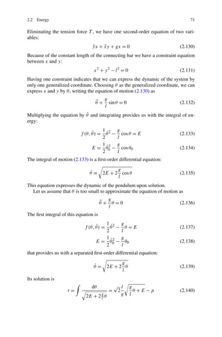
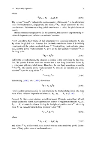
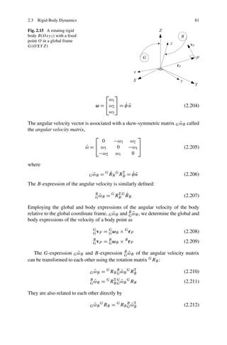
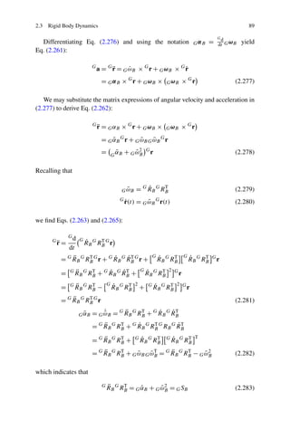
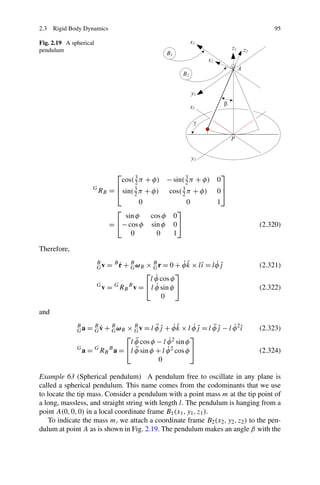
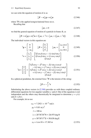
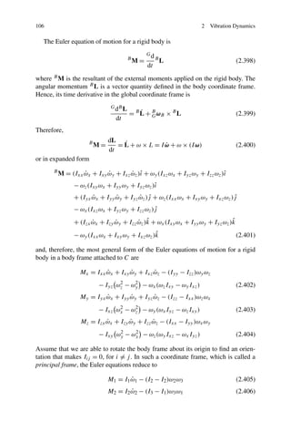
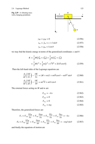
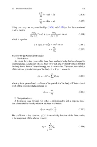
![144 2 Vibration Dynamics
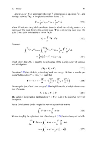
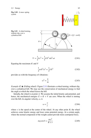
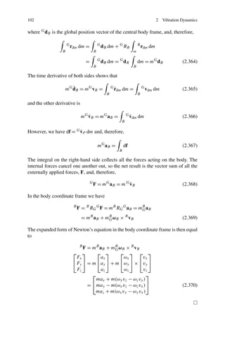
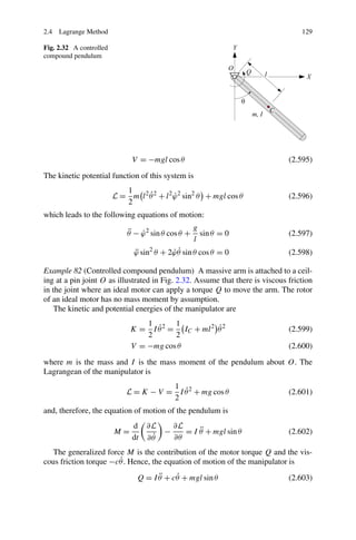
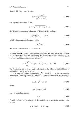
Fig. 2.38 A quarter car
model with driver
1
[c] = [k] + [k]T (2.726)
2
1
[k] = [c] + [c]T (2.727)
2
From now on, we assume that every equation of motion is found from the La-
grange method to have symmetric coefficient matrices. Hence, we show the equa-
tions of motion, thus:
[m]¨ + [c]˙ + [k]x = F
x x (2.728)
and use [m], [c], [k] as a substitute for [m], [c], [k]:
[m] ≡ [m] (2.729)
[c] ≡ [c] (2.730)
[k] ≡ [k] (2.731)
Symmetric matrices are equal to their transpose:
[m] ≡ [m]T (2.732)
[c] ≡ [c] T
(2.733)
[k] ≡ [k]T (2.734)
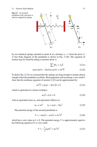
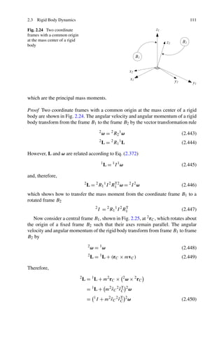
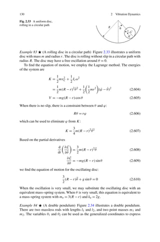
Example 91 (A quarter car model with driver’s chair) Figure 2.38 illustrates a
quarter car model plus a driver, which is modeled by a mass md over a linear cushion
above the sprung mass ms .](https://image.slidesharecdn.com/advancedvibrations-130411024927-phpapp01/85/Advanced-vibrations-94-320.jpg)
![2.6 Quadratures 145
Assuming
y=0 (2.735)
we find the free vibration equations of motion. The kinetic energy K of the system
can be expressed by
1 1 1
K = mu xu + ms xs + md xd
˙2 ˙2 ˙2
2 2 2
⎡ ⎤⎡ ⎤
mu 0 0 ˙
xu
1
= xu xs xd ⎣ 0 ms 0 ⎦ ⎣ xs ⎦
˙ ˙ ˙ ˙
2 0 0 md ˙
xd
1
˙
= xT [m]˙
x (2.736)
2
and the potential energy V can be expressed as
1 1 1
V = ku (xu )2 + ks (xs − xu )2 + kd (xd − xs )2
2 2 2
⎡ ⎤⎡ ⎤
ku + ks −ks 0 xu
1
= xu xs xd ⎣ −ks ks + kd −kd ⎦ ⎣ xs ⎦
2 0 −k k x
d d d
1
= xT [k]x (2.737)
2
Similarly, the dissipation function D can be expressed by
1 1 1
D = cu (xu )2 + cs (xs − xu )2 + cd (xd − xs )2
˙ ˙ ˙ ˙ ˙
2 2 2
⎡ ⎤⎡ ⎤
cu + cs −cs 0 ˙
xu
1
= xu xs xd ⎣ −cs
˙ ˙ ˙ cs + cd −cd ⎦ ⎣ xs ⎦
˙
2 0 −c c ˙
x
d d d
1
˙
= xT [c]˙
x (2.738)
2
Employing the quadrature derivative method, we may find the derivatives of K, V ,
and D with respect to their variable vectors:
⎡ ⎤
˙
xu
∂K 1 1 T ⎣ ⎦
˙
= [m] + [m] x = [k] + [k]
T
˙
xs
∂x ˙ 2 2 ˙
x d
⎡ ⎤⎡ ⎤
mu 0 0 ˙
xu
=⎣ 0 ms 0 ⎦ ⎣ xs ⎦
˙ (2.739)
0 0 md ˙
xd](https://image.slidesharecdn.com/advancedvibrations-130411024927-phpapp01/85/Advanced-vibrations-95-320.jpg)
![146 2 Vibration Dynamics
⎡ ⎤
xu
∂V 1 1
= [k] + [k]T x = [k] + [k]T ⎣ xs ⎦
∂x 2 2 xd
⎡ ⎤⎡ ⎤
ku + ks −ks 0 xu
= ⎣ −ks ks + kd −kd ⎦ ⎣ xs ⎦ (2.740)
0 −kd kd xd
∂D 1
˙
= [c] + [c]T x
˙
∂x 2
⎡ ⎤
˙
xu
1
= [c] + [c]T ⎣ xs ⎦
˙
2 ˙
x d
⎡ ⎤⎡ ⎤
cu + cs −cs 0 ˙
xu
= ⎣ −cs cs + cd −cd ⎦ ⎣ xs ⎦
˙ (2.741)
0 −cd cd ˙
xd
Therefore, we find the system’s free vibration equations of motion:
[m]¨ + [c]˙ + [k]x = 0
x x (2.742)
⎡ ⎤⎡ ⎤ ⎡ ⎤⎡ ⎤
mu 0 0 ¨
xu cu + cs −cs 0 ˙
xu
⎣0 ms 0 ⎦ ⎣ xs ⎦ + ⎣ −cs
¨ cs + cd −cd ⎦ ⎣ xs ⎦
˙
0 0 md ¨
xd 0 −cd cd ˙
xd
⎡ ⎤⎡ ⎤
ku + ks −ks 0 xu
+ ⎣ −ks ks + kd −kd ⎦ ⎣ xs ⎦ = 0 (2.743)
0 −kd kd xd
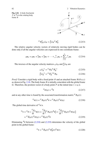
Example 92 (Different [m], [c], and [k] arrangements) Mass, damping, and stiff-
ness matrices [m], [c], [k] for a vibrating system may be arranged in different forms
with the same overall kinetic energy K, potential energy V , and dissipation function
D. For example, the potential energy V for the quarter car model that is shown in
Fig. 2.38 may be expressed by different [k]:
1 1 1
V = ku (xu )2 + ks (xs − xu )2 + kd (xd − xs )2 (2.744)
2 2 2
⎡ ⎤
ku + ks −ks 0
1
V = xT ⎣ −ks ks + kd −kd ⎦ x (2.745)
2 0 −k kd
d
⎡ ⎤
k + ks −2ks 0
1 T⎣ u
V= x 0 ks + kd −2kd ⎦ x (2.746)
2 0 0 kd](https://image.slidesharecdn.com/advancedvibrations-130411024927-phpapp01/85/Advanced-vibrations-96-320.jpg)
![2.6 Quadratures 147
⎡ ⎤
k + ks 0 0
1 T⎣ u
V= x −2ks ks + kd 0 ⎦x (2.747)
2 0 −2kd kd
The matrices [m], [c], and [k], in K, D, and V , may not be symmetric; however,
˙ ˙
the matrices [m], [c], and [k] in ∂K/∂ x, ∂D/∂ x, ∂V /∂x are always symmetric.
When a matrix [a] is diagonal, it is symmetric and
[a] = [a] (2.748)
A diagonal matrix cannot be written in different forms. The matrix [m] in Exam-
ple 91 is diagonal and, hence, K has only one form, (2.736).
Example 93 (Quadratic form and sum of squares) We can write the sum of xi2 in the
quadratic form,
n
xi2 = xT x = xT I x (2.749)
i=1
where
xT = x1 x2 x3 · · · xn (2.750)
and I is an n × n identity matrix. If we are looking for the sum of squares around a
mean value x0 , then
n n n n
1
(xi − x0 )2 = xi2 − nx0 = xT x −
2
xi xi
n
i=1 i=1 i=1 i=1
1 T
= xT x − x 1n 1T x
n
n
1
= xT I − 1n 1T x
n (2.751)
n
where
1T = 1 1
n ··· 1 (2.752)
Example 94 (Positive definite matrix) A matrix [a] is called positive definite if
xT [a]x > 0 for all x = 0. A matrix [a] is called positive semidefinite if xT [a]x ≥ 0
for all x.
The kinetic energy is positive definite, and this means we cannot have K = 0
˙
unless x = 0. The potential energy is positive semidefinite and this means that we
have V ≥ 0 as long as x > 0; however, it is possible to have a especial x0 > 0 at
which V = 0.
A positive definite matrix, such as the mass matrix [m], satisfies Silvester’s crite-
rion, which is that the determinant of [m] and determinant of all the diagonal minors](https://image.slidesharecdn.com/advancedvibrations-130411024927-phpapp01/85/Advanced-vibrations-97-320.jpg)
![148 2 Vibration Dynamics
must be positive:
m11 m12 ··· m1n
m21 m22 ··· m2n
Δn = . .. .. . >0
.
. . . .
.
mn1 mn2 ··· mnn
m11 m12 ··· m1,n−1
m21 m22 ··· m2,n−1
Δn−1 = . .. .. . >0
.
. . . .
.
mn1 mn2 ··· mn−1,n−1
m11 m12
· · · Δ2 = >0 Δ1 = m11 > 0 (2.753)
m21 m22
Example 95 (Symmetric matrices) Employing the Lagrange method guarantees
that the coefficient matrices of equations of motion of linear vibrating systems are
symmetric. A matrix [A] is symmetric if the columns and rows of [A] are inter-
changeable, so [A] is equal to its transpose:
[A] = [A]T (2.754)
The characteristic equation of a symmetric matrix [A] is a polynomial for which
all the roots are real. Therefore, the eigenvalues of [A] are real and distinct and [A]
is diagonalizable.
Any two eigenvectors that come from distinct eigenvalues of the symmetric ma-
trix [A] are orthogonal.
Example 96 (Linearization of energies) The kinetic energy of a system with n par-
ticles is
n 3n
1 1
K= mi xi2 + yi2 + zi =
˙ ˙ ˙2 ˙i
mi u2 (2.755)
2 2
i=1 i=1
Expressing the configuration coordinate ui in terms of generalized coordinates qj ,
we have
n
∂ui ∂ui
˙
ui = qs +
˙ s = 1, 2, . . . , N (2.756)
∂qs ∂t
s=1](https://image.slidesharecdn.com/advancedvibrations-130411024927-phpapp01/85/Advanced-vibrations-98-320.jpg)
![150 2 Vibration Dynamics
n n N
1 ∂ui ∂ui
K2 = mi ˙ ˙
qj qk (2.765)
2 ∂qj ∂qk
j =1 k=1 i=1
where
N N
∂ui ∂ui ˙ ˙
∂ ui ∂ ui
akj = aj k = mi = mi (2.766)
∂qk ∂qj ˙ ˙
∂ qk ∂ qj
i=1 i=1
If the coordinates ui do not depend explicitly on time t, then ∂ui /∂t = 0, and we
have
n n n n
1 1 ∂ 2 K(0)
K = K2 = aj k qj qk =
˙ ˙ ˙ ˙
qj qk
2 2 ∂qj ∂qi
j =1 k=1 j =1 k=1
n n
1
= ˙ ˙
mij qj qk (2.767)
2
j =1 k=1
The kinetic energy is a scalar quantity and, because of (2.755), must be positive
definite. The first term of (2.757) is a positive quadratic form. The third term of
(2.757) is also a nonnegative quantity, as indicated by (2.760). The second term of
˙
(2.755) can be negative for some qj and t. However, because of (2.755), the sum of
all three terms of (2.757) must be positive:
1
˙ ˙
K = qT [m]q (2.768)
2
The generalized coordinate qi represent deviations from equilibrium. The poten-
tial energy V is a continuous function of generalized coordinates qi and, hence, its
expansion is
n n n
∂V (0) 1 ∂ 2 V (0)
V (q) = V (0) + qi + qi qj + · · · (2.769)
∂qi 2 ∂qj ∂qi
i=1 j =1 i=1
where ∂V (0)/∂qi and ∂ 2 V (0)/(∂qj ∂qi ) are the values of ∂V /∂qi and ∂ 2 V /(∂qj ∂qi )
at q = 0, respectively. By assuming V (0) = 0, and knowing that the first derivative
of V is zero at equilibrium
∂V
= 0 i = 1, 2, 3, . . . , n (2.770)
∂qi
we have the second-order approximation
n n
1
V (q) = kij qi qj (2.771)
2
j =1 i=1](https://image.slidesharecdn.com/advancedvibrations-130411024927-phpapp01/85/Advanced-vibrations-100-320.jpg)
![2.7 Variational Dynamics 151
∂ 2 V (0)
kij = (2.772)
∂qj ∂qi
where kij are the elastic coefficients. The second-order approximation of V is zero
only at q = 0. The expression (2.771) can also be written as a quadrature:
1
V = qT [k]q (2.773)
2
2.7 Variational Dynamics
˙
Consider a function f of x(t), x(t), and t:
f = f (x, x, t)
˙ (2.774)
The unknown variable x(t), which is a function of the independent variable t, is
called a path. Let us assume that the path is connecting the fixed points x0 and xf
during a given time t = tf − t0 . So x = x(t) satisfies the boundary conditions
x(t0 ) = x0 x(tf ) = xf (2.775)
The time integral of the function f over x0 ≤ x ≤ xf is J (x) such that its value
depends on the path x(t):
tf
J (x) = ˙
f (x, x, t) dt (2.776)
t0
where J (x) is called an objective function or a functional.
The particular path x(t) that minimizes J (x) must satisfy the following equation:
∂f d ∂f
− =0 (2.777)
∂x dt ∂ x˙
This equation is the Lagrange or Euler–Lagrange differential equation and is in
general of second order.
Proof To show that a path x = x (t) is a minimizing path for the functional J (x) =
tf
˙
t0 f (x, x, t) dt with boundary conditions (2.775), we need to show that
J (x) ≥ J x (2.778)
for all continuous paths x(t). Any path x(t) satisfying the boundary conditions
(2.775) is called an admissible path. To see that x (t) is the optimal path, we may
examine the integral J for every admissible path. Let us define an admissible path
by superposing another admissible path y(t) onto x ,
x(t) = x + y(t) (2.779)](https://image.slidesharecdn.com/advancedvibrations-130411024927-phpapp01/85/Advanced-vibrations-101-320.jpg)
![2.8 Key Symbols 161
Using a similar treatment of the successive pairs of terms of (2.851), we derive the
following n conditions to minimize (2.841):
∂f d ∂f
− = 0 i = 1, 2, . . . , n (2.854)
∂qi ˙
dt ∂ qi
Therefore, when a definite integral is given which contains n functions to be deter-
mined by the condition that the integral be stationary, we can vary these functions
independently. So, the Euler–Lagrange equation can be formed for each function
separately. This provides us with n differential equations.
2.8 Key Symbols
a≡x ¨ acceleration
a, b distance, Fourier series coefficients
a, b, w, h length
a acceleration
A, B weight factor, coefficients for frequency responses
c damping
[c] damping matrix
ce equivalent damping
C mass center
d position vector of the body coordinate frame
df infinitesimal force
dm infinitesimal mass
dm infinitesimal moment
E mechanical energy, Young modulus of elasticity
f = 1/T cyclic frequency [Hz]
f, F, f, F force
FC Coriolis force
g gravitational acceleration
H height
I moment of inertia matrix
I1 , I2 , I3 principal moment of inertia
k stiffness
ke equivalent stiffness
kij element of row i and column j of a stiffness matrix
[k] stiffness matrix
K kinetic energy
l directional line
L moment of momentum
L=K −V Lagrangean
m mass
me eccentric mass, equivalent mass](https://image.slidesharecdn.com/advancedvibrations-130411024927-phpapp01/85/Advanced-vibrations-111-320.jpg)
![162 2 Vibration Dynamics
mij element of row i and column j of a mass matrix
mk spring mass
ms sprung mass
[m] mass matrix
n number of coils, number of decibels, number of note
N natural numbers
p pitch of a coil
P power
r frequency ratio
r position vector
t time
t0 initial time
T period
Tn natural period
v ≡ x, v
˙ velocity
V potential energy
x, y, z, x displacement
x0 initial displacement
˙
x0 initial velocity
˙ ˙ ˙
x, y, z velocity, time derivative of x, y, z
x¨ acceleration
X amplitude of x
z relative displacement
Greek
α, β, γ angle, angle of spring with respect to displacement
δ deflection, angle
δs static deflection
ε mass ratio
θ angular motion coordinate
ω, ω, Ω angular frequency
ϕ, Φ phase angle
λ eigenvalue
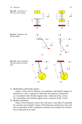
2.9 Exercises
1. Equation of motion of vibrating systems.
Determine the equation of motion of the systems in Figs. 2.41(a) and (b) by
(a) using the energy method
(b) using the Newton method
(c) using the Lagrange method](https://image.slidesharecdn.com/advancedvibrations-130411024927-phpapp01/85/Advanced-vibrations-112-320.jpg)
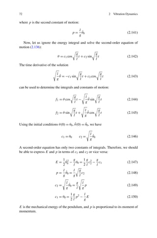
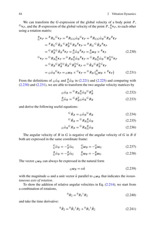
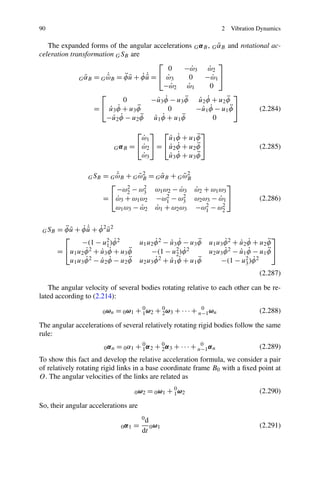
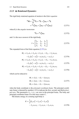
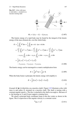
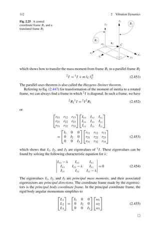
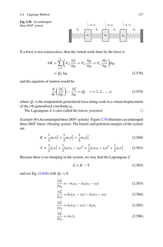
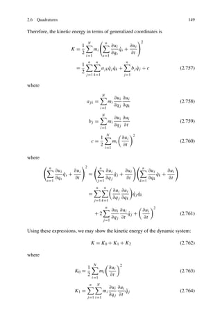
![168 2 Vibration Dynamics
Fig. 2.51 (a) A slender as a
pendulum with variable
density. (b) A simple
pendulum with the same
length
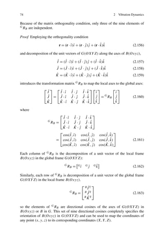
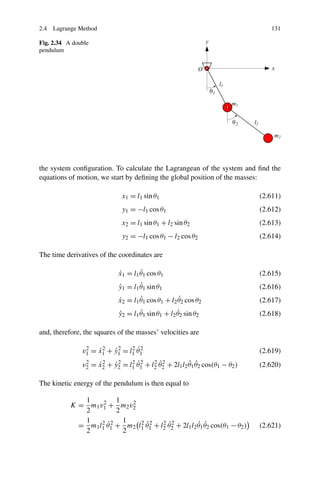
Fig. 2.52 Four connected
pendulums
Fig. 2.53 Two spring
connected heavy discs
17. Variable density.
Figure 2.51(a) illustrates a slender as a pendulum with variable density, and
Fig. 2.51(b) illustrates a simple pendulum with the same length. Determine the
equivalent mass me is the mass density ρ = m/ l is
(a) ρ = C1 z
(b) ρ = C2 (l − z)
(c) ρ = C3 (z − 2 )2
l
(d) ρ = C4 ( 2 − (z − 2 ))2
l l
18. Four pendulums are connected as shown in Fig. 2.52.
(a) Determine the kinetic energy K, linearize the equation and find the mass
matrix [m].
(b) Determine the potential energy V , linearize the equation and find the stiff-
ness matrix [k].
(c) Determine the equations of motion using K and V and determine the sym-
metric matrices [m] and [k].
19. Two spring connected heavy discs.
The two spring connected disc system of Fig. 2.53 is linear for small θ1
and θ2 . Find the equations of motion by energy and Lagrange methods.](https://image.slidesharecdn.com/advancedvibrations-130411024927-phpapp01/85/Advanced-vibrations-118-320.jpg)

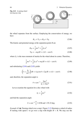
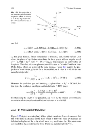
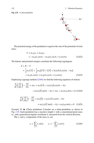
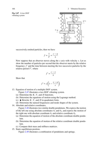
This chapter discusses vibration dynamics and methods for deriving equations of motion. The Newton-Euler and Lagrange methods are commonly used to derive equations of motion for vibrating systems. The Newton-Euler method is well-suited for discrete, lumped parameter models with a low degree of freedom. It involves drawing free body diagrams and applying Newton's second law to each mass to obtain the equations of motion. Having symmetric coefficient matrices is the main advantage of using the Lagrange method for mechanical vibrations.


