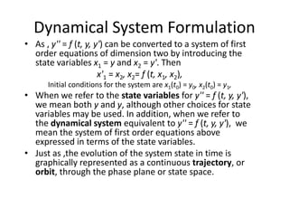
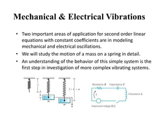
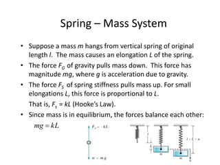
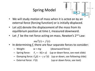
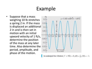
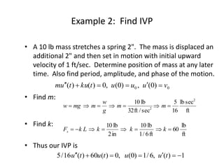
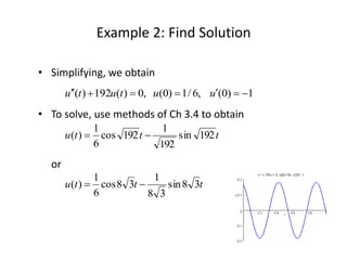
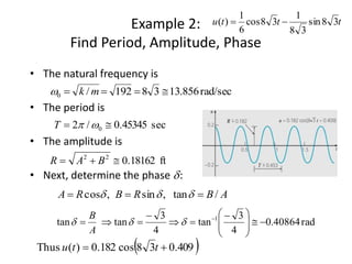
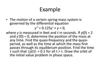
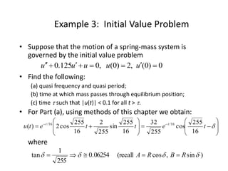
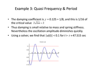
The document introduces second order differential equations and their solutions. It defines an initial value problem for a second order equation as consisting of the equation and two initial conditions. Linear equations are introduced, which can be written in standard form or with constant or variable coefficients. The dynamical system formulation converts a second order equation to a system of first order equations. Undamped and damped free vibrations are discussed. Examples are provided, including finding the solution to an initial value problem, and determining the quasi-frequency, quasi-period, and equilibrium crossing time.

2. INTRODUCTION
A second order differential equation is an equation
involving the independent variable
t, and an unknown function or dependent variable y =
y(t) along with its first and second
derivatives. We will assume that it is always possible
to solve for the second derivative so
that the equation has the form
y'' = f (t, y, y'),
A solution of it on an interval I is a function y = φ(t),
twice continuously differentiable on I, such that φ''(t)
= f (t, φ(t), φ'(t)) for all values of t ∈ I.

3. Definitions and Examples
• An initial value problem for a second order
equation on an interval I consists of y'' = f (t, y,
y'), together with two initial conditions y(t0) =
y0, y'(t0) = y1, prescribed at a point t0 ∈ I,
where y0 and y1 are any given numbers.
• Thus y = φ(t) is a solution of the initial value
problem on I if, in addition to satisfying y'' = f
(t, y, y') on I, φ(t0) = y0 and φ'(t0) = y1.

4. Linear Equations
• The differential equation y'' = f (t, y, y') is said to
be linear if it can be written in the standard
form
y'' + p(t) y' + q(t)y = g(t), (A)
where the coefficient of y'' is equal to 1. The
coefficients p, q, and g can be arbitrary
functions of the independent variable t, but y,
y', and y'' can appear in no other way except as
designated by the form of Eq. (A).
• Equation (A) is said to be homogeneous if the term g(t)
is zero for all t. Otherwise the equation is
nonhomogeneous, and the term g(t) is referred to as
the nonhomogeneous term.

5. Linear Equations
• A slightly more general form of a linear second order
equation is
P(t)y'' + Q(t)y' + R(t)y = G(t).
• This Equation is said to be a constant coefficient
equation if P, Q, and R are constants. In this case, Eq.
reduces to
ay'' + by' + cy = g(t)
where a = 0, b, and c are given constants and we have
replaced G(t) by g(t).
• Otherwise Eq. has variable coefficients.

6. Dynamical System Formulation
• As , y'' = f (t, y, y') can be converted to a system of first
order equations of dimension two by introducing the
state variables x1 = y and x2 = y'. Then
x'1 = x2, x2= f (t, x1, x2),
Initial conditions for the system are x1(t0) = y0, x2(t0) = y1,
• When we refer to the state variables for y'' = f (t, y, y'),
we mean both y and y, although other choices for state
variables may be used. In addition, when we refer to
the dynamical system equivalent to y'' = f (t, y, y'), we
mean the system of first order equations above
expressed in terms of the state variables.
• Just as ,the evolution of the system state in time is
graphically represented as a continuous trajectory, or
orbit, through the phase plane or state space.

7. Mechanical & Electrical Vibrations
• Two important areas of application for second order linear
equations with constant coefficients are in modeling
mechanical and electrical oscillations.
• We will study the motion of a mass on a spring in detail.
• An understanding of the behavior of this simple system is the
first step in investigation of more complex vibrating systems.

8. Spring – Mass System
• Suppose a mass m hangs from vertical spring of original
length l. The mass causes an elongation L of the spring.
• The force FG of gravity pulls mass down. This force has
magnitude mg, where g is acceleration due to gravity.
• The force FS of spring stiffness pulls mass up. For small
elongations L, this force is proportional to L.
That is, Fs = kL (Hooke’s Law).
• Since mass is in equilibrium, the forces balance each other:
kLmg 

9. Spring Model
• We will study motion of mass when it is acted on by an
external force (forcing function) or is initially displaced.
• Let u(t) denote the displacement of the mass from its
equilibrium position at time t, measured downward.
• Let f be the net force acting on mass. Newton’s 2nd Law:
• In determining f, there are four separate forces to consider:
– Weight: w = mg (downward force)
– Spring force: Fs = - k(L+ u) (up or down force, see next slide)
– Damping force: Fd(t) = -  u (t) (up or down, see following slide)
– External force: F(t) (up or down force, see text)
)()( tftum 

10. Spring Model:
Spring Force Details
• The spring force Fs acts to restore spring to natural position,
and is proportional to L + u. If L + u > 0, then spring is
extended and the spring force acts upward. In this case
• If L + u < 0, then spring is compressed a distance of |L + u|,
and the spring force acts downward. In this case
• In either case,
)( uLkFs 
    uLkuLkuLkFs 
)( uLkFs 

11. TYPES OF OSCILLATIONS
• Undamped Free oscillations
Recall that the equation of motion for the damped spring-
mass system with external forcing is
my'' + γ y' + ky = F(t)
with initial conditions, y(0) = y0, y(0) = v0, that specify initial
position y0 and initial velocity v0 provide a complete
formulation of the vibration problem.
• If there is no external force, then F(t) = 0. Assume that
there is no damping, so γ = 0.
• We get my'' + ky = 0. If we divide by m, it becomes
y'' + ω2
0 y = 0,
where ω2
0 = k/m.

12. Undamped Free Vibrations
• The characteristic equation for diff. eq. is
λ2 + ω2
0 = 0, and the corresponding characteristic roots
are λ=±ω0. It follows that the general solutionis
y = A cos ω0t + B sin ω0t.
Via the initial conditions to determine the integration
constants A and B in terms of initial position and
velocity,
A = y0 and B = v0/ ω0.
• We can write y in the phase amplitude form
y = R cos(ω0t − δ).

13. Undamped Free Vibrations
• The period of the motion isT = 2π/ω0= 2π(m/k)1/2.
• The circular frequency ω0 =√(k/m), measured in
radians per unit time, is called the natural frequency
of the vibration.
• The maximum displacement R of the mass from
equilibrium is the amplitude of the motion.
• The dimensionless parameter δ is called the phase,
or phase angle, and measures the displacement of
the wave from its normal position corresponding to δ
= 0.

14. Example
• Suppose that a mass
weighing 10 lb stretches
a spring 2 in. If the mass
is displaced an additional
2 in and is then set in
motion with an initial
upward velocity of 1 ft/s,
determine the position
of the mass at any later
time. Also determine the
period, amplitude, and
phase of the motion.

15. Example 2: Find IVP
• A 10 lb mass stretches a spring 2". The mass is displaced an
additional 2" and then set in motion with initial upward
velocity of 1 ft/sec. Determine position of mass at any later
time. Also find period, amplitude, and phase of the motion.
• Find m:
• Find k:
• Thus our IVP is
ft
seclb
16
5
sec/ft32
lb10 2
2
 mm
g
w
mmgw
ft
lb
60
ft6/1
lb10
in2
lb10
 kkkLkFs
1)(,6/1)0(,0)(60)(16/5  tuututu
00 )0(,)0(,0)()( vuuutkutum 

16. Example 2: Find Solution
• Simplifying, we obtain
• To solve, use methods of Ch 3.4 to obtain
or
1)0(,6/1)0(,0)(192)(  uututu
tttu 192sin
192
1
192cos
6
1
)( 
tttu 38sin
38
1
38cos
6
1
)( 

17. Example 2:
Find Period, Amplitude, Phase
• The natural frequency is
• The period is
• The amplitude is
• Next, determine the phase :
tttu 38sin
38
1
38cos
6
1
)( 
rad/sec856.1338192/0  mk
sec45345.0/2 0  T
ft18162.022
 BAR
rad40864.0
4
3
tan
4
3
tantan 1







 


 

A
B
ABRBRA /tan,sin,cos  
 409.038cos182.0)(Thus  ttu

18. Damped Free Vibrations
• If we include the effect of damping, the differential equation
governing the motion of the mass is my''+γy'+ky=0.
• The roots of the corresponding characteristic equation,
mλ2+γλ+k=0 leads to 3 cases.
• 1. Underdamped Harmonic Motion (γ2−4km < 0).
The roots are μ ±iν with μ = −γ/2m < 0 and ν = (4km − γ2)1/2/2m>
0 and general solution is y = e−γt/2m(A cos νt + B sin νt).
• 2. CriticallyDampedHarmonic Motion (γ2−4km =0).
In this case, λ1=−γ/2m<0 is a repeated root and the general
solution is y = (A + Bt)e−γt/2m

19. Damped Free Vibrations
• 3. Overdamped Harmonic Motion (γ2−4km > 0).
In this case, the values of λ1 and λ2 are real, distinct,
and negative, and the general solution is y = Aeλ1t +
Beλ2t.
• The most important case is the first one, which
occurs when the damping is small. If we let A = R cos
δ and B = R sin δ, then we obtain
y = Re−γ t/2m cos(νt − δ).
ν is called the quasi-frequency and Td = 2π/ν is called
the quasi-period.

20. Example
• The motion of a certain spring-mass system is
governed by the differential equation
y'' + 0.125y' + y = 0,
where y is measured in feet and t in seconds. If y(0) = 2
and y'(0) = 0, determine the position of the mass at
any time. Find the quasi-frequency and the quasi-
period, as well as the time at which the mass first
passes through its equilibrium position. Find the time
τ such that |y(t)| < 0.1 for all t > τ. Draw the orbit of
the initial value problem in phase space.

21. Example 3: Initial Value Problem
• Suppose that the motion of a spring-mass system is
governed by the initial value problem
• Find the following:
(a) quasi frequency and quasi period;
(b) time at which mass passes through equilibrium position;
(c) time  such that |u(t)| < 0.1 for all t > .
• For Part (a), using methods of this chapter we obtain:
where
0)0(,2)0(,0125.0  uuuuu
















 
tettetu tt
16
255
cos
255
32
16
255
sin
255
2
16
255
cos2)( 16/16/
)sin,cos(recall06254.0
255
1
tan  RBRA 

22. Example 3: Quasi Frequency & Period
• The solution to the initial value problem is:
• The graph of this solution, along with solution to the
corresponding undamped problem, is given below.
• The quasi frequency is
and quasi period
• For undamped case:
















 
tettetu tt
16
255
cos
255
32
16
255
sin
255
2
16
255
cos2)( 16/16/
998.016/255 
295.6/2  dT
283.62,10   T

23. Example 3: Quasi Frequency & Period
• The damping coefficient is  = 0.125 = 1/8, and this is 1/16 of
the critical value
• Thus damping is small relative to mass and spring stiffness.
Nevertheless the oscillation amplitude diminishes quickly.
• Using a solver, we find that |u(t)| < 0.1 for t >   47.515 sec
22 km

24. Example 3: Quasi Frequency & Period
• To find the time at which the mass first passes through the
equilibrium position, we must solve
• Or more simply, solve
0
16
255
cos
255
32
)( 16/








 
tetu t
sec637.1
2255
16
216
255












t
t