1. This document contains solutions to problems from Chapter 1 of the textbook "The Physics of Vibrations and Waves".
2. It provides detailed calculations and explanations for problems related to simple harmonic motion, including determining restoring forces, stiffness, frequencies, and solving differential equations of motion.
3. Examples include a simple pendulum, a mass on a spring, and vibrations of strings, membranes, and gas columns.
![x = + a 2 for the first time after release, the value of ωt is the minimum
solution of equation asin(ωt −π 2) = + a 2 , i.e. ωt = 3π 4 . Similarly, we can
find: for x = a 2 , ωt = 2π 3 and for x = 0 , ωt =π 2 .
If the solution x = acos(ωt +φ ) satisfies x = −a at t = 0 , then,
x = a cosφ = −a i.e. φ =π . When the pendulum swings to the position
x = + a 2 for the first time after release, the value of ωt is the minimum
solution of equation acos(ωt +π ) = + a 2 , i.e. ωt = 3π 4 . Similarly, we can
find: for x = a 2 , ωt = 2π 3 and for x = 0 , ωt =π 2 .
If the solution x = asin(ωt −φ ) satisfies x = −a at t = 0 , then,
x = asin(−φ ) = −a i.e. φ =π 2 . When the pendulum swings to the position
x = + a 2 for the first time after release, the value of ωt is the minimum
solution of equation asin(ωt −π 2) = + a 2 , i.e. ωt = 3π 4 . Similarly, we can
find: for x = a 2 , ωt = 2π 3 and for x = 0 , ωt =π 2 .
If the solution x = a cos(ωt −φ ) satisfies x = −a at t = 0 , then,
x = acos(−φ ) = −a i.e. φ =π . When the pendulum swings to the position
x = + a 2 for the first time after release, the value of ωt is the minimum
solution of equation acos(ωt −π ) = + a 2 , i.e. ωt = 3π 4 . Similarly, we can
find: for x = a 2 , ωt = 2π 3 and for x = 0 , ωt =π 2 .
1.4
The frequency of such a simple harmonic motion is given by:
s
e
πε π
e e = = = rad s
© 2008 John Wiley & Sons, Ltd
4.5 10 [ ]
19 2
−
(1.6 ×
10 )
4 8.85 10 (0.05 10 ) 9.1 10
4
16 1
12 9 3 31
3
0
2
0
−
− − −
≈ × ⋅
× × × × × × ×
r m
m
ω
Its radiation generates an electromagnetic wave with a wavelength λ given by:](https://image.slidesharecdn.com/136253314-physics-of-vibration-and-waves-solutions-pain-141001200006-phpapp01/85/physics-of-vibration-and-waves-solutions-pain-6-320.jpg)
![= = − π
ω
© 2008 John Wiley & Sons, Ltd
c ≈ × m = nm
2 2 3 10 8
4.2 10 [ ] 42[ ]
× × ×
16
4.5 10
8
0
×
π
λ
Therefore such a radiation is found in X-ray region of electromagnetic spectrum.
1.5
(a) If the mass m is displaced a distance of x from its equilibrium position, either
the upper or the lower string has an extension of x 2 . So, the restoring force of
the mass is given by: F = −sx 2 and the stiffness of the system is given by:
s′ = −F x = s 2 . Hence the frequency is given by s m s m a ω2 = ′ = 2 .
(b) The frequency of the system is given by: s m b ω2 =
(c) If the mass m is displaced a distance of x from its equilibrium position, the
restoring force of the mass is given by: F = −sx − sx = −2sx and the stiffness of
the system is given by: s′ = −F x = 2s . Hence the frequency is given by
s m s m c ω2 = ′ =2 .
Therefore, we have the relation: 2 : 2 : 2 = s 2m: s m: 2s m = 1: 2 : 4 a b c ω ω ω
1.6
At time t = 0 , 0 x = x gives:
0 asinφ = x (1.6.1)
0 x& = v gives:
0 aω cosφ = v (1.6.2)
From (1.6.1) and (1.6.2), we have
0 0 tanφ =ωx v and 2 2 1 2
a = (x 2
+ v ω )
0 0
1.7
The equation of this simple harmonic motion can be written as: x = asin(ωt +φ ) .
The time spent in moving from x to x + dx is given by: t dt = dx v , where t v is
the velocity of the particle at time t and is given by: v = x = aω cos(ωt +φ ) t & .](https://image.slidesharecdn.com/136253314-physics-of-vibration-and-waves-solutions-pain-141001200006-phpapp01/85/physics-of-vibration-and-waves-solutions-pain-7-320.jpg)
![Noting that the particle will appear twice between x and x + dx within one period
of oscillation. We have the probability η of finding it between x to x + dx given
by:
η = 2dt where the period is given by:
T
dt
2 2
ω
© 2008 John Wiley & Sons, Ltd
2π T = , so we have:
ω
dx
dx
dx
dx
2 cos( ) cos( ) a 1 sin2 ( t
) a 2 x
2
a t
a t
T
−
=
− +
=
+
=
+
= =
π ω ω φ π ω φ π ω φ π
η
1.8
Since the displacements of the equally spaced oscillators in y direction is a sine
curve, the phase difference δφ between two oscillators a distance x apart given is
proportional to the phase difference 2π between two oscillators a distance λ apart
by: δφ 2π = x λ , i.e. δφ = 2πx λ .
1.9
The mass loses contact with the platform when the system is moving downwards and
the acceleration of the platform equals the acceleration of gravity. The acceleration of
a simple harmonic vibration can be written as: a = Aω 2 sin(ωt +φ ) , where A is the
amplitude, ω is the angular frequency and φ is the initial phase. So we have:
Aω 2 sin(ωt +φ ) = g
i.e.
ω 2 sin(ω +φ )
=
t
A g
Therefore, the minimum amplitude, which makes the mass lose contact with the
platform, is given by:
A g g ≈
min 2 4 2 2 2 2 m
0.01[ ]
9.8
= = =
ω π π
4 5
f
× ×
1.10
The mass of the element dy is given by: m′ = mdy l . The velocity of an element
dy of its length is proportional to its distance y from the fixed end of the spring, and
is given by: v′ = yv l . where v is the velocity of the element at the other end of the
spring, i.e. the velocity of the suspended mass M . Hence we have the kinetic energy](https://image.slidesharecdn.com/136253314-physics-of-vibration-and-waves-solutions-pain-141001200006-phpapp01/85/physics-of-vibration-and-waves-solutions-pain-8-320.jpg)
![⎛
y
− + ⎟ ⎟⎠
x
y
sin sin cos cos
2
φ φ φ φ
2
2
⎞
xy
x
y
xy
y
x
sin sin 2 sin sin cos cos 2 cos cos
⎛
x
= + − + + −
φ φ φ φ φ φ φ φ
2
xy
y
(sin cos ) (sin cos ) 2 (sin sin cos cos )
x
= + + + − +
2
2
2
2
φ φ φ φ φ φ φ φ
xy
y
x
= + − −
© 2008 John Wiley & Sons, Ltd
E = 1 mx& 2 + 1
sx 2
(1.12.4)
2
2
Write (1.12.3) in form x&2 =ω2 (a2 − x2 ) and substitute into (1.12.4), then we have:
E = 1 mx& + 1
sx = 1
mω ( a − x ) + 1
sx
2 2 2 2 2 2
2
2
2
2
Noting that the frequency ω is given by: ω 2 = s m , we have:
E = 1 s a − x + sx = 1
sa
( ) 1
2
2 2 2 2
2
2
which is a constant value.
1.13
The equations of the two simple harmonic oscillations can be written as:
sin( ) 1 y = a ωt +φ and sin( ) 2 y = a ωt +φ +δ
The resulting superposition amplitude is given by:
[sin( ) sin( )] 2 sin( 2)cos( 2) 1 2 R = y + y = a ωt +φ + ωt +φ +δ = a ωt +φ +δ δ
and the intensity is given by:
I = R2 = 4a2 cos2 (δ 2)sin2 (ωt +φ +δ 2)
i.e. I ∝ 4a2 cos2 (δ 2)
Noting that sin2 (ωt +φ +δ 2) varies between 0 and 1, we have:
0 ≤ I ≤ 4a2 cos2 (δ 2)
1.14
2 cos( )
1 2
1 2
2
2
2
1
1 2 1 2
1 2
1
2
1
2
2
2
2
2
2
2
2
1
1 2
1 2
2
2
2
1
1
2
2
2
1 2
1 2
1
2
2
2
2
2
2
1
2
2
1
1
2
2
1
2
2
1
φ φ
⎟ ⎟⎠
⎜ ⎜⎝
⎞
⎜ ⎜⎝
−
a a
a
a
a a
a
a
a a
a
a
a a
a
a
a
a
a
a
On the other hand, by substitution of :
x = +
1 1
1
sinωt cosφ cosωt sinφ
a](https://image.slidesharecdn.com/136253314-physics-of-vibration-and-waves-solutions-pain-141001200006-phpapp01/85/physics-of-vibration-and-waves-solutions-pain-12-320.jpg)
![m(xy& − yx&) = m(−abω sin2ωt − abω cos2ωt) = −abmω(sin2ωt + cos2ωt) = −abmω
which is a constant. The quantity abmω is the angular momentum of the particle.
1.16
All possible paths described by equation 1.3 fall within a rectangle of 1 2a wide and
2 2a high, where 1 max a = x and 2 max a = y , see Figure 1.8.
When x = 0 in equation (1.3) the positive value of sin( ) 2 2 1 y = a φ −φ . The value of
max 2 y = a . So sin( ) 0 max 2 1 = φ −φ = y y x which defines 2 1 φ −φ .
1.17
In the range 0 ≤φ ≤π , the values of i cosφ are −1 ≤ cos ≤ +1 i φ
© 2008 John Wiley & Sons, Ltd
. For n random
values of i φ , statistically there will be n 2 values −1 ≤ cos ≤ 0 i φ
and n 2 values
0 ≤ cos ≤ 1 i φ
. The positive and negative values will tend to cancel each other and the
n
Σ →
sum of the n values: cos 0
i i
1
j ≠ =
i φ
→ Σ=
, similarly cos 0
1
n
j
j φ
. i.e.
Σ Σ →
cos cos 0
1 =
1
≠ =
n
j
j
n
j i i
i φ φ
1.18
The exponential form of the expression:
a sinωt + a sin(ωt +δ ) + a sin(ωt + 2δ ) +L+ a sin[ωt + (n −1)δ ]
is given by:
aeiωt + aei(ωt+δ ) + aei(ωt+2δ ) +L+ aei[ωt+(n−1)δ ]
From the analysis in page 28, the above expression can be rearranged as:
⎡
⎞
⎛ −
+
ae ω δ nδ
2 sin 2
sin 2
1
δ
i t n ⎥⎦
⎤
⎢⎣
⎟⎠
⎜⎝
with the imaginary part:
δ ω n n t a ⎥⎦
sin δ
2
sin 2
⎡
−
sin +
⎛ 1
2
δ
⎤
⎢⎣
⎞
⎟⎠
⎜⎝
which is the value of the original expression in sine term.](https://image.slidesharecdn.com/136253314-physics-of-vibration-and-waves-solutions-pain-141001200006-phpapp01/85/physics-of-vibration-and-waves-solutions-pain-14-320.jpg)
![where 1 C is arbitrary in value. Use initial condition, we get 1 0 C = q ,
i.e. q = q e−t RC 0
which shows the relaxation time of the process is RC s.
2.5
(a) 2 2 2
2 2 -6
0 ω -ω′ =10 ω = r 4m => 500 0 ω m r =
π
1 2 4 3
E = mx&2 + sx2 = sx = × × − = × − J
E E E −
© 2008 John Wiley & Sons, Ltd
0
ω′ ≈ , so:
The condition also shows 0 ω
500 0 Q =ω′m r ≈ω m r =
Use
ω
τ
′
′ = 2
, we have:
π π
r
π
r
δ τ = =
′
2 ω
500
= ′ =
m Q
m
(b) The stiffness of the system is given by:
2 1012 10 10 100[ 1]
0
s =ω m = × − = Nm−
and the resistive constant is given by:
6 10
10 10 7 1
r m ω
0 − −
2 10 [ ]
500
−
= × ⋅
×
= = N sm
Q
(c) At t = 0 and maximum displacement, x& = 0 , energy is given by:
100 10 5 10 [ ]
1
2
1
2
1
2
2
max
Time for energy to decay to e−1of initial value is given by:
0.5[ ]
t m 10
=
= = −
2 10
7
10
ms
r
×
−
(d) Use definition of Q factor:
E
Q E
− Δ
= 2π
where, E is energy stored in system, and − ΔE is energy lost per cycle, so energy loss in the
first cycle, 1 − ΔE , is given by:
2 2 5 10 5
2 10 [ ]
500
3
1 J
Q
−
= ×
×
− Δ = −Δ = π = π × π
2.6](https://image.slidesharecdn.com/136253314-physics-of-vibration-and-waves-solutions-pain-141001200006-phpapp01/85/physics-of-vibration-and-waves-solutions-pain-18-320.jpg)
![2
− +
ω ω
1 1 ( ) 2 2 2 2 2
ε χ cos
r ω
© 2008 John Wiley & Sons, Ltd
ne m
( )
2 2 2 2 2
0
2
ω −
ω
[ ( ) ]
0
2 2
0
2
nex
E
ε m ω ω ω
r
0 ε
χ
− +
= − =
So we have:
t
ne m
m r
[ ( ) ]
ε ω ω ω
0
2
0
2 −
2
0
= + = +
3.11
The instantaneous power dissipated is equal to the product of frictional force and the
instantaneous velocity, i.e.:
2
P rx x r F
( ) cos2 ( )
= = 0 ωt −φ
2
Z
m
& &
The period for a given frequency ω is given by:
2π T =
ω
Therefore, the energy dissipated per cycle is given by:
2
0
E Pdt r F
∫ ∫
= = −
2
0
rF
π ω
2
0 2
= − −
rF
2
0
π
ω
rF
2
2
0
2
0
2
0
2
2
2
2
ω φ
[1 cos2( )]
2
cos ( )
m
m
m
T
m
π
Z
Z
t dt
Z
t dt
Z
ω
ω φ
π ω
=
=
∫
(3.11.1)
The displacement is given by:
x F
= t −
0 sin(ω φ )
ω
Z
m
so we have:
x F
max = (3.11.2)
m Z
ω
0
By substitution of (3.11.2) into (3.11.1), we have:
2
max E =πrωx
3.12
The low frequency limit of the bandwidth of the resonance absorption curve 1 ω
satisfies the equation:](https://image.slidesharecdn.com/136253314-physics-of-vibration-and-waves-solutions-pain-141001200006-phpapp01/85/physics-of-vibration-and-waves-solutions-pain-30-320.jpg)
![LC R C LC R C −
2 1
0 ω = ,
Q 0L
0
© 2008 John Wiley & Sons, Ltd
0
1 2
2
LV
0 =
⎞
⎟⎠
ω
+ ⎛ −
⎜⎝
C
R L
d
d
ω
ω
ω
i.e. 1 1 0
2 2
2 2
2
⎞
+ ⎛ −
2 = + − ⎟⎠
⎜⎝
C
L
C
R L
ω
ω
ω
ω
L
i.e. 2 + 2 − 2 =
0
2 2
C
C
R
ω
i.e.
2
0
0
2
0
1 1
2 2 2 0 2
R
2
1 1
2
2
1
1
2
1
2
1
Q
L
L
=
−
=
−
=
−
=
ω
ω
ω ω
where
LC
ω
=
R
3.16
Considering an electron in an atom as a lightly damped simple harmonic oscillator,
we know its resonance absorption bandwidth is given by:
δω = r (3.16.1)
m
On the other hand, the relation between frequency and wavelength of light is given
by:
f = c (3.16.2)
λ
where, c is speed of light in vacuum. From (3.16.2) we find at frequency resonance:
f = − c
δ 20
δλ
λ
where 0 λ
is the wavelength at frequency resonance. Then, the relation between
angular frequency bandwidth δω and the width of spectral line δλ is given by:
π
= 2 f = 2 c δλ
(3.16.3)
δω π δ 20
λ
From (3.16.1) and (3.16.3) we have:
r λ
r
0
δλ = = 0
=
m Q
λ
cm
0
20
2
λ
ω
π
So the width of the spectral line from such an atom is given by:
−
= ×
0.6 10 −
14
1.2 10 [ ]
×
5 10
7
6
λ
0 m
Q
×
= =
δλ](https://image.slidesharecdn.com/136253314-physics-of-vibration-and-waves-solutions-pain-141001200006-phpapp01/85/physics-of-vibration-and-waves-solutions-pain-34-320.jpg)
![Provided x is the extension of the spring and l is the natural length of the spring,
we have:
2 2 13 2 27 2
s m m
(2 ) 4 × (1.14 × 10 ) × (23 × 35) × (1.67 ×
10 ) 1
Na Cl πν π
2 −
= = Nm
m m
© 2008 John Wiley & Sons, Ltd
x − x = l + x 2 1
By elimination of 1 x and 2 x , we have:
s − − = &&
x s
x x
m
m
2 1
x& m +
m
&i.e. 0
+ sx
m m
1 2 =
1 2
which shows the system oscillate at a frequency:
ω2 = s
μ
where,
m m
+
1 2
m m
1 2
μ =
For a sodium chloride molecule the interatomic force constant s is given by:
120[ ]
(23 35) 1.67 10
27
−
−
≈
+ × ×
=
+
Na Cl
ω μ
4.5
If the upper mass oscillate with a displacement of x and the lower mass oscillate
with a displacement of y , the equations of motion of the two masses are given by
Newton’s second law as:
mx s ( y x )
sx
= − −
&&
my s x y
( )
= −
&&
i.e.
mx s x y sx
&&
( ) 0
− − =
+ − − =
my s x y
( ) 0
&&
Suppose the system starts from rest and oscillates in only one of its normal modes of
frequency ω , we may assume the solutions:
i t
ω
i t
x =
Ae
y Be
ω
=
where A and B are the displacement amplitude of x and y at frequency ω .](https://image.slidesharecdn.com/136253314-physics-of-vibration-and-waves-solutions-pain-141001200006-phpapp01/85/physics-of-vibration-and-waves-solutions-pain-40-320.jpg)
![Using these solutions, the equations of motion become:
x 2 a cos ( )
t t 2 1 1 2
a t t
2 sin ( )
© 2008 John Wiley & Sons, Ltd
2
m A s A B sA e
[ − ω
+ ( − ) + ] =
0
2
i t
[ − − ( − )] =
0
i t
m B s A B e
ω
ω
ω
We may, by dividing through by meiωt , rewrite the above equations in matrix form
as:
0
2
2
2
A
⎤
= ⎥⎦
⎡
⎢⎣
⎤
⎥⎦
⎡
⎢⎣
s m − −
s m
− −
B
s m s m
ω
ω
(4.5.1)
which has a non-zero solution if and only if the determinant of the matrix vanishes;
that is, if
(2s m−ω 2 )(s m−ω2 ) − s2 m2 = 0
i.e. ω 4 − (3s m)ω 2 + s2 m2 = 0
i.e.
s
2
m
ω 2 = (3± 5)
In the slower mode, ω 2 = (3 − 5) s 2m . By substitution of the value of frequency
into equation (4.5.1), we have:
5 1
2
A ω
2
2
2
−
=
s −
m
=
−
=
s
s
s m
B
ω
which is the ratio of the amplitude of the upper mass to that of the lower mass.
Similarly, in the slower mode, ω 2 = (3 + 5) s 2m . By substitution of the value of
frequency into equation (4.5.1), we have:
5 1
2
A ω
2
2
2
+
= −
s −
m
=
−
=
s
s
s m
B
ω
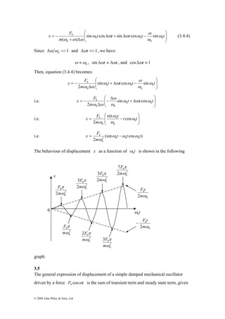
4.6
The motions of the two pendulums in Figure 4.3 are given by:
m a
cos ( )
y a t t a ω t ω
t
m a
sin ( )
ω ω ω ω
ω ω
ω ω ω ω
2 sin sin
2
2
2 cos cos
2
2
2 1 1 2
=
− +
=
=
− +
=
a ω
where, the amplitude of the two masses, 2 a cosω t and 2 a sinω t , are constants
m m over one cycle at the frequency .
Supposing the spring is very weak, the stiffness of the spring is ignorable, i.e. s ≈ 0.](https://image.slidesharecdn.com/136253314-physics-of-vibration-and-waves-solutions-pain-141001200006-phpapp01/85/physics-of-vibration-and-waves-solutions-pain-41-320.jpg)
![Noting that 2 = g l
1 ω
E s a 1
mg
2 2 2 2 2
= = =
ω ω ω
1
x x x m a m
E = ma ω ω − ω t = E + ω −
ω
t
x a
= − = − −
© 2008 John Wiley & Sons, Ltd
and 2 ( 2 )
2 ω = g l + s m , we have:
g ω
2
2
⎛ +
ω ω
2 1 2
2
2
⎞
= ≈ ≈
ω ω = ⎟⎠
⎜⎝
l 1 2 a
Hence, the energies of the masses are given by:
( )
( a t) ma t
l
E s a mg
a t ma t
l
1
2 2 2 2 2
2 sin 2 sin
ω ω ω
1
y y y m a m
2
2
2 cos 2 cos
2
2
= = =
The total energy is given by:
2 2 2 (cos2 sin2 ) 2 2 2 x y a m m a E = E + E = ma ω ω t + ω t = ma ω
Noting that ( ) 2 2 1 ω = ω −ω m , we have:
[1 cos( ) ]
2
2 sin ( )
[1 cos( ) ]
2
2 cos ( )
ω ω ω ω ω
2 1 2 1
2 2 2
2 1 2 1
2 2 2
E ma t E t
y a
which show that the constant energy E is completed exchanged between the two
pendulums at the beat frequency ( ) 2 1 ω −ω .
4.7
By adding up the two equations of motion, we have:
( )( ) 1 2 1 2 m &x&+m &y& = − m x +m y g l
By multiplying the equation by 1 ( ) 1 2 m +m on both sides, we have:
m x +
m y
1 2
l
1 2
m x m y
&&+ &&
1 2
1 2
m m
g
m m
+
= −
+
m x +
m y
l
m &x& +
m &y&
i.e. 1 2 1 2
=
0
1 2
1 2
+
+
+
m m
g
m m
which can be written as:
2 0
1 X&& +ω X = (4.7.1)
where,
X m x +
m y
= and 2 = g l
1 2
m +
m
1 2
1 ω](https://image.slidesharecdn.com/136253314-physics-of-vibration-and-waves-solutions-pain-141001200006-phpapp01/85/physics-of-vibration-and-waves-solutions-pain-42-320.jpg)
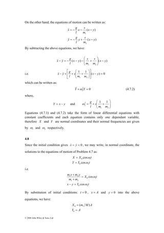
![where, 1 2 M = m +m
so the equations of motion in original coordinates x , y are given by:
[ cos( ω ω ) cos( ω ω
) ]
= − + +
a m a m
1 2
[ (cos ω cos ω sin ω sin ω ) (cos ω cos ω sin ω sin ω
)]
= + + −
m a m a m a m a
1 2
m m t t m m t t
x A
A
A
[( )cos ω cos ω ( )sin ω sin ω
]
= + + −
m a m a
1 2 1 2
A t t A
cos cos ( )sin sin
ω ω ω ω
= + −
E 1
m x s x m x mg
x m x m ω
x
l
= & + = & + = &
+
x x a
E 1
m y s y m y mg
= + = + = +
© 2008 John Wiley & Sons, Ltd
m
A t
M
m x +
m y
1 2
m m
x y A t
2
1
1
1 2
cos
cos
ω
ω
− =
=
+
The solutions to the above equations are given by:
m t m t
( cos ω cos ω
)
= +
(cos cos )
1 2
x A
y A m
1
1 1 2 2
t t
M
M
ω ω
= −
Noting that a m ω =ω −ω 1 and a m ω =ω +ω 2 , where ( ) 2 2 1 ω = ω −ω m and
( ) 2 1 2 ω = ω +ω a , the above equations can be rearranged as:
m m t t
M
M
m t t t t m t t t t
M
m t m t
M
m a 1 2
m a
and
[cos( ) cos( ) ]
= − − +
ω ω ω ω
a m a m
t t
y A m
A m
2 sin sin
M
t t
M
ω ω
m a
1
1
=
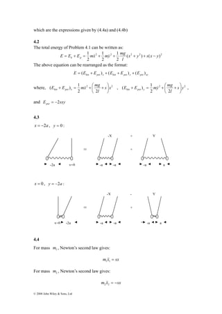
4.9
From the analysis in Problem 4.6, we know, at weak coupling conditions, t m cosω
and t m sinω are constants over one cycle, and the relation: g l a ω ≈ , so the energy
of the mass 1 m , x E , and the energy of the mass 2 m , y E , are the sums of their
separate kinetic and potential energies, i.e.:
2 2
ω
1
2
& & &
1
1
1
2 2
2
1
1
2 2
21
2 2
1
2
1
2 2
1
2 2
1
1
2
1
2
2
1
2
2
2
1
2
1
2
2
1
2
2
2
y m y m y
l
y y a](https://image.slidesharecdn.com/136253314-physics-of-vibration-and-waves-solutions-pain-141001200006-phpapp01/85/physics-of-vibration-and-waves-solutions-pain-44-320.jpg)
![By substitution of the expressions of x and y in terms of t acosω and t a ω
E 1
m A t t A
= ⎡− + −
ω ω ω ω ω ω
x a m a a m a
m A t t A
⎡ + −
ω ω ω ω ω
a m a m a
m A
2
= + + −
ω ω ω
a m m
m A
2
= + + −
ω ω ω
a m m
m A
1
1
1
1
E
ω ω
= + + −
E m A m
2 sin cos 1
1
+ ⎡ ⎥⎦
ω ω ω ω ω ω
= ⎡
y a m a a m a
m m A
2
2 ω sin ω (cos ω sin ω
)
= +
a m a a
m m A
2
2 sin
ω ω
a m
m A m m
1
⎞
⎛
2 2 1 2
⎞
ω ω
= ⎛
E m m
1 2
= ⎛
m(x y) mg ( ) ( ) 2 ( ) cosω 0 &&− && + − + & − & + − =
© 2008 John Wiley & Sons, Ltd
sin
given by Problem 4.8 into the above equations, we have:
[ ]
[ ]
[ 2 cos2
]
2
[m m m m t]
M
m m m m t
M
m m m m t t
M
m m t m m t
M
m m t t
M
m m t t
M
a m
2 cos( )
2
2 (cos sin )
2
( ) cos ( ) sin
2
cos cos ( )sin sin
2
cos sin ( )sin cos
2
1 2 2 1
2
2
2
2 1
1 2
2
2
2
2 1
2
1
2 2
1 2
2
2
2
2 1
2
1
2 2
1 2
2 2
2 1 2
2
1
2
1 2
2
1
2
1 1 2
ω ω
= + +
⎤
⎥⎦
⎢⎣
⎤
+ ⎥⎦
⎢⎣
and
t t m A m
[ ]
2 1 cos2
[ ]
2
⎞
⎟⎠
[ t]
M
t
M
t
M
t t t
M
t t
M
M
a m
2 1 cos( )
2
2 sin sin
2
2
2 2 1
1
2
2
2
2
2
1
2 2 2
2
2
2
2
1
2
2 1
1
2
1
2
ω ω
− − ⎟⎠
⎜⎝
− ⎟⎠
⎜⎝
⎜⎝
=
⎤
⎥⎦
⎢⎣
⎤
⎢⎣
where,
E 1 m A a ω
2 2
2 1
=
4.10
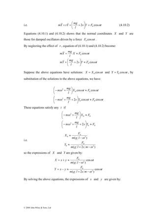
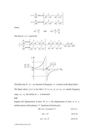
Add up the two equations and we have:
m(&&+ x && y) + mg ( x + y ) + r ( x & + y & ) =
F cosω t
0 l
mX rX mg cosω 0 && + & + = (4.10.1)
i.e. X F t
l
Subtract the two equations and we have:
x y r x y s x y F t
l](https://image.slidesharecdn.com/136253314-physics-of-vibration-and-waves-solutions-pain-141001200006-phpapp01/85/physics-of-vibration-and-waves-solutions-pain-45-320.jpg)
![− = −
− = − − + −
© 2008 John Wiley & Sons, Ltd
mx s y x
( )
= −
&&
My s y x s z y
( ) ( )
= − − + −
&&
mz s z y
( )
= − −
&&
If the system has a normal frequency of ω , and the displacements of the three masses
can by written as:
i t
ω
i t
x η
e
1
=
y e
ω
i t
η
2
=
z e
ω
η
3
=
By substitution of the expressions of displacements into the above equations of
motion, we have:
i t i t
ω ω
m e s e
( )
ω η η η
i t i t i t
ω ω ω
M e s e s e
( ) ( )
ω η η η η η
i t i t
ω ω
m e s e
( )
ω η η η
3 3 2
2
2 2 1 3 2
2
1 2 1
2
− = − −
i.e.
s m s e
[( − ω ) η − η
] =
0
s s M s e
[ − η + (2 − ω ) η − η
] =
0
i t
[ ( ) ] 0
3
2
2
2 3
2
1
1 2
2
− + − =
i t
i t
s s m e
ω
ω
ω
η ω η
which is true for all t if
s m s
( − ω ) η − η
=
0
s s M s
(2 ) 0
− η + − ω η − η
=
s s m
( ) 0
3
2
2
2 3
2
1
1 2
2
− η + − ω η
=
The matrix format of these equations is given by:
0
s − m −
s
s s M s
− − −
0
2
0
η
1
η
2
3
2
2
2
=
⎞
⎟ ⎟ ⎟
⎠
⎞
⎛
⎟ ⎟ ⎟
⎜ ⎜ ⎜
⎝
⎠
⎛
⎜ ⎜ ⎜
⎝
− −
η
ω
ω
ω
s s m
which has non zero solutions if and only if the determinant of the matrix is zero, i.e.:
(s −mω2 )2 (2s −Mω 2 ) − 2s2 (s −mω2 ) = 0
i.e. (s −mω2 )[(s −mω 2 )(2s −Mω 2 ) − 2s2 ] = 0
i.e. (s −mω2 )[mMω 4 − s(M + 2m)ω 2 ] = 0
i.e. ω2 (s −mω2 )[mMω 2 − s(M + 2m)] = 0
The solutions to the above equation, i.e. the frequencies of the normal modes, are
given by:
2 0
1 ω = ,
2 = s
m
2 ω
and
2 s(M +
2m)
3
mM
ω =](https://image.slidesharecdn.com/136253314-physics-of-vibration-and-waves-solutions-pain-141001200006-phpapp01/85/physics-of-vibration-and-waves-solutions-pain-54-320.jpg)
![SOLUTIONS TO CHAPTER 5
5.1
Write u = ct + x , and try 2
2
1
∂
© 2008 John Wiley & Sons, Ltd
2
x
y
∂
∂
with ( ) 2 y = f ct + x , we have:
f u
2 f ( u
)
∂ ( ) 2 , and 2
u
y
x
∂
∂
=
∂
2
2
2
u
x
y
∂
∂
=
∂
∂
Try 2
2
t
y
c ∂
with ( ) 2 y = f ct + x , we have:
c f u
2 ( )
c f u
∂ ( ) 2 , and 2
u
y
t
∂
∂
=
∂
2
2
2
2
u
t
y
∂
∂
=
∂
∂
so:
f u
c f u
y
1 1 ( ) ( )
2
2
2
2
2
2
2
2 2
2
2
∂
c ∂
u
u
t c
∂
=
∂
∂
=
∂
Therefore:
2
2
2 y
1
2 2
t
y
x c
∂
∂
=
∂
∂
5.2
If ( ) 1 y = f ct − x , the expression for y at a time t + Δt and a position x + Δx , where
Δt = Δx c , is given by:
y f c t t x x
[ ( ) ( )]
= + Δ − + Δ +Δ +Δ
, 1
f c t x c x x
[ ( ) ( )]
= + Δ − + Δ
1
f ct x x x
[ ]
= + Δ − − Δ
t x
t t x x
1
f [ ct x ]
y
= − =
1 ,
i.e. the wave profile remains unchanged.
If ( ) 2 y = f ct + x , the expression for y at a time t + Δt and a position x + Δx , where
Δt = −Δx c , is given by:](https://image.slidesharecdn.com/136253314-physics-of-vibration-and-waves-solutions-pain-141001200006-phpapp01/85/physics-of-vibration-and-waves-solutions-pain-58-320.jpg)
![y
c y
x
y
∂
=
∂
t
∂
∂
© 2008 John Wiley & Sons, Ltd
y f c t t x x
[ ( ) ( )]
= + Δ + + Δ +Δ +Δ
, 1
f c t x c x x
[ ( ) ( )]
= − Δ + + Δ
1
f ct x x x
[ ]
= − Δ + + Δ
t x
t t x x
1
f [ ct x ]
y
= + =
1 ,
i.e. the wave profile also remains unchanged.
5.3
5.4
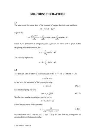
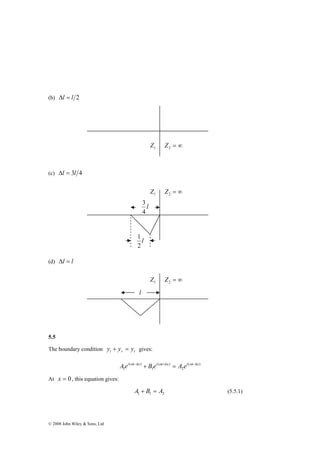
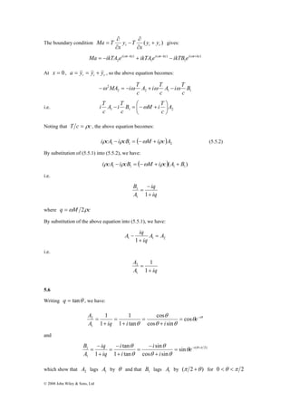
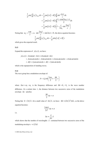
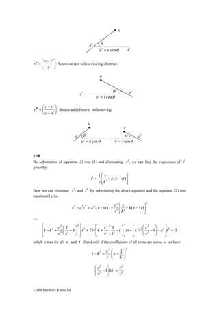
The pulse shape before reflection is given by the graph below:
The pulse shapes after of a length of Δl of the pulse being reflected are shown below:
(a) Δl = l 4
x
x
l
l
2
3
l
4
1
1 Z = ∞ 2 Z](https://image.slidesharecdn.com/136253314-physics-of-vibration-and-waves-solutions-pain-141001200006-phpapp01/85/physics-of-vibration-and-waves-solutions-pain-59-320.jpg)
![The reflected energy coefficients are given by:
2
0
ω
∫ ∫
W = − T − ka t − kx a t −
kx dxdt
k a T π ω
k
t kx dxdt
∫ ∫
= −
k a T t kx dxdt
2 2 2
= ⋅ ⋅ ⋅
F T y ω
max sin( )
© 2008 John Wiley & Sons, Ltd
θ (θ π 2) 2 2θ
2
B
1 = sin e−i + = sin
A
1
and the transmitted energy coefficients are given by:
θ θ 2 2θ
2
A
2 = cos e−i = cos
A
1
5.7
Suppose T is the tension of the string, the average rate of working by the force over one period
of oscillation on one-wavelength-long string is given by:
∂
y
x
∂
∂
ω 2
= − π ω
∫ ∫ ∂
π
0
1
2 0
dxdt
t
W T y k
By substitution of y = asin(ωt − kx) into the above equation, we have:
2
1
1 cos(2 2 )
2 1
2
2
2
2
sin ( )
2
[ sin( )][ sin( )]
2
2
2
0
1
0
2 2 2
2
0
1
0
2
2 2 2
1
0
ka T
k
k a T
k
k
ω
π
ω
π
ω
ω
π
ω
ω
π
ω
ω ω ω
π
π ω
π ω
=
− −
=
∫ ∫
Noting that k =ω c and T = ρc2 , the above equation becomes
2 2 2 2a2 c
c
W ω a ρ c ω ρ
= =
2 2
which equals the rate of energy transfer along the string.
5.8
Suppose the wave equation is given by: y = sin(ωt − kx) . The maximum value of transverse
harmonic force max F is given by:
A t kx TAk TA
x
c
T
⎛
∂
x
⎤
⎡ −
∂
ω = = ⎥⎦
⎢⎣
∂
⎞
= ⎟⎠
⎜⎝
∂
=
max max
i.e.](https://image.slidesharecdn.com/136253314-physics-of-vibration-and-waves-solutions-pain-141001200006-phpapp01/85/physics-of-vibration-and-waves-solutions-pain-62-320.jpg)
![P ρ ω
π
= c A = T = × × × × =
c P
1 R
1 θ
1 θ
2 θ
© 2008 John Wiley & Sons, Ltd
0.3
0.3 max =
0.1 × 2 ×
5
= =
A
ω π π
F
T
c
Noting that ρc = T c , the rate of energy transfer along the string is given by:
0.3 (2 5) 0.1 3
[ ]
20
1
2
1
2
2
2 2 2 2
2 2
A W
c
π
π
ω
so the velocity of the wave c is given by:
2 2 3 20 1
2 2 2 2
30[ ]
×
π
= = ms
0.01 (2 5) 0.1
= −
× × ×
A
π π
ρω
5.9
This problem is not viable in its present form and it will be revised in the next printing. The first
part in the zero reflected amplitude may be solved by replacing Z3 by Z1, which then equates r
with R′ because each is a reflection at a 1 2 Z Z boundary. We then have the total reflected
amplitude as:
2
R tTR R 2 R 4
R tTR
1
(1 )
− ′
R
′
+ ′ + ′ + ′ +L = +
Stokes’ relations show that the incident amplitude may be reconstructed by reversing the paths of
the transmitted and reflected amplitudes.
T is transmitted back along the incident direction as tT in 1 Z and is reflected as TR′ in
2 Z .
R is reflected in 1 Z as (R)R = R2 back along the incident direction and is refracted as TR
in the TR′ direction in 2 Z .
We therefore have tT + R2 = 1 in 1 Z , i.e. tT = 1− R2 and T(R + R′) = 0 in 2 Z giving
R = −R′ , ∴tT = 1− R2 = 1− R′2 giving the total reflected amplitude in 1 Z as R + R′ = 0
with R = −R′ .
T
R2
tT R
1 θ
1 θ
TR′ θ
θ
2 2 T TR
Fig Q.5.9(a) Fig Q.5.9(b)
1 Z
2 Z
1 Z](https://image.slidesharecdn.com/136253314-physics-of-vibration-and-waves-solutions-pain-141001200006-phpapp01/85/physics-of-vibration-and-waves-solutions-pain-63-320.jpg)
![Note that for zero total reflection in medium Z1, the first reflection R is cancelled by the sum of all
subsequent reflections.
5.10
The impedance of the anti-reflection coating coat Z should have a relation to the impedance of air
air Z and the impedance of the lens lens Z given by:
2
2
y n n
∂
k n ω
= , we have:
© 2008 John Wiley & Sons, Ltd
Z = Z Z = 1
coat air lens n n
air lens
So the reflective index of the coating is given by:
= 1 = = 1.5 = 1.22 air lens
coat n n
coat
Z
n
and the thickness of the coating d should be a quarter of light wavelength in the coating, i.e.
1.12 10 [ ]
5.5 ×
10
4 1.22
4
7
7
m
λ
n
d
coat
−
−
= ×
×
= =
5.11
By substitution of equation (5.10) into
y
∂
∂
x
, we have:
y n
A t B t t
ω
= ( cos + sin )cos
n ω
c
∂
x c
ω ω
n n n n
∂
so:
y
A t B t t
c c
x c
n n n n
n
2
2
2
2
( cos sin )sin
ω ω
ω ω
ω
= − + = −
∂
Noting that
c
2
2
+ = − + =
∂
∂ y
0 2
2
2
2
2
c
y
c
k y
x
y n n ω ω
5.12
By substitution of the expression of max
( 2 ) n y into the integral, we have:](https://image.slidesharecdn.com/136253314-physics-of-vibration-and-waves-solutions-pain-141001200006-phpapp01/85/physics-of-vibration-and-waves-solutions-pain-64-320.jpg)
![e n
= = × × rad s
ω
v
© 2008 John Wiley & Sons, Ltd
2 2 c2k 2 e ω =ω + (5.17.1)
As e ω
ω → , we have:
2
⎞
= − ⎛
ωe
1 1
2
2
< ⎟⎠
⎜⎝
ω
c
v
i.e. v > c , which means the phase velocity exceeds that of light c .
From equation (5.17.1), we have:
d( 2 ) d( 2 c2k 2 ) e ω = ω +
i.e. 2ωdω = 2kc2dk
which shows the group velocity g v is given by:
v = d = = = c
<
g c c
v
c k c
v
dk
2
2
ω
ω
i.e. the group velocity is always less than c .
5.18
From equation (5.17.1), we know that only electromagnetic waves of e ωω > can propagate
through the electron plasma media.
For an electron number density ~ 1020 e n , the electron plasma frequency is given by:
20
1.6 10 − 10 = × 11 ⋅
1
5.65 10 [ ]
31 12
9.1 10 8.8 10
19
0
−
− −
× × ×
m
e
e
e ε
Now consider the wavelength of the wave in the media given by:
2 2 2 2 3 10 3
3 10 [ ]
11
× ×
5.65 10
8
v v c m
f
π
π
e e
= × −
×
π
= = < < =
π
ω
ω
ω
λ
which shows the wavelength has an upper limit of 3×10⁻³m.
5.19
The dispersion relation ω 2 c2 = k 2 + m2c2 h2 gives
d(ω 2 c2 ) = d(k 2 + m2c2 h2 )
2 ω
ω =
2
2 i.e. d kdk
c](https://image.slidesharecdn.com/136253314-physics-of-vibration-and-waves-solutions-pain-141001200006-phpapp01/85/physics-of-vibration-and-waves-solutions-pain-67-320.jpg)
![d
k
i.e. c2
⎞
⎛
T
2 1 1 2 15 1 13 1
⎞
⎛
T
2 1 1 2 15 1 13 1
© 2008 John Wiley & Sons, Ltd
dk
=
ω ω
Noting that the group velocity is dω dk and the particle (phase) velocity is ω k , the above
equation shows their product is c2 .
5.20
The series in the problem is that at the bottom of page 132. The frequency components can be
expressed as:
R na t ω
t
sin( ω
2)
Δ ⋅
t
ω
cos
2
Δ ⋅
=
which is a symmetric function to the average frequency 0 ω
. It shows that at
Δt = 2 , R = 0 ,
π
Δ
ω
∴Δt ⋅Δω = 2π
In k space, we may write the series as:
y(k) a cos k x a cos(k k)x a cos[k (n 1) k]x 1 1 1 = + +δ +L+ + − δ
As an analogy to the above analysis, we may replace ω by k and t by x , and R is zero at
k
x
Δ
Δ =
2π
, i.e. ΔkΔx = 2π
5.21
The frequency of infrared absorption of NaCl is given by:
3.608 10 [ ]
1
35 1.66 10
23 1.66 10
27 27
−
⎞
− − ⋅ × = ⎟⎠
⎛
⎜⎝
× ×
+
× ×
× × = ⎟ ⎟⎠
⎜ ⎜⎝
= + rad s
a m m
Na Cl
ω
The corresponding wavelength is given by:
52[ ]
2 2 × 3 ×
10
λ ≈
13
3.608 10
8
c π
μm
π
ω
×
= =
which is close to the experimental value: 61μm
The frequency of infrared absorption of KCl is given by:
3.13 10 [ ]
1
35 1.66 10
39 1.66 10
27 27
−
⎞
− − ⋅ × = ⎟⎠
⎛
⎜⎝
× ×
+
× ×
× × = ⎟ ⎟⎠
⎜ ⎜⎝
= + rad s
a m m
K Cl
ω
The corresponding wavelength is given by:
60[ ]
2 2 × 3 ×
10
λ ≈
13
3.13 10
8
c π
μm
π
ω
×
= =
which is close to the experimental value: 71μm](https://image.slidesharecdn.com/136253314-physics-of-vibration-and-waves-solutions-pain-141001200006-phpapp01/85/physics-of-vibration-and-waves-solutions-pain-68-320.jpg)
![5.22
Before the source passes by the observer, the source has a velocity of u , the frequency noted by
the observer is given by:
′ = ν
ν can be written in the format of wavelength as:
© 2008 John Wiley & Sons, Ltd
c
−
ν ν
c u
= 1
After the source passes by the observer, the source has a velocity of − u , the frequency noted by
the observer is given by:
c
+
ν ν
c u
= 2
So the change of frequency noted by the observer is given by:
2
cu
c
c
⎞
⎛
2 1 c2 u2
( )
c u
c u
−
= ⎟⎠
⎜⎝
+
−
−
Δ = − =
ν
ν ν ν ν
5.23
By superimposing a velocity of − v on the system, the observer becomes stationary and the
source has a velocity of u − v and the wave has a velocity of c − v . So the frequency registered
by the observer is given by:
c v
c v
−
−
ν ν
c u
c v u v
−
=
− − −
′′′ =
( )
5.24
The relation between wavelength λ and frequency ν of light is given by:
ν = c
λ
So the Doppler Effect
c
−
c u
2
c u
c c
( −
)
=
λ′ λ
c − u
i.e. λ λ
c
′ =
Noting that wavelength shift is towards red, i.e. λ′ > λ , so we have:
Δ = ′ − = − u
λ λ λ λ
c
8 11
u = − c Kms
3 × 10 ×
10 1
λ
i.e. 5[ ]
6 10
7
−
−
−
= −
×
= −
Δ
λ
which shows the earth and the star are separating at a velocity of 5Kms−1 .
5.25](https://image.slidesharecdn.com/136253314-physics-of-vibration-and-waves-solutions-pain-141001200006-phpapp01/85/physics-of-vibration-and-waves-solutions-pain-69-320.jpg)
![Suppose the aircraft is flying at a speed of u , and the signal is being transmitted from the aircraft
at a frequency of ν and registered at the distant point at a frequency of ν ′ . Then, the Doppler
Effect gives:
′′ −
ν
ν ν
u = c c ms
−
T mNau ≈
v vc ⎞
: Observer is at rest with a moving source.
⎛
− ′
© 2008 John Wiley & Sons, Ltd
c
−
c u
ν ′ =ν
Now, let the distant point be the source, reflecting a frequency of ν ′ and the flying aircraft be the
receiver, registering a frequency of ν ′′ . By superimposing a velocity of − u on the flying
aircraft, the distant point and signal waves, we bring the aircraft to rest; the distant point now has a
velocity of − u and signal waves a velocity of − c − u . Then, the Doppler Effect gives:
c +
u
c u
c u
′ − − ν ′′ =ν ν ν
c
c u
c u u
−
=
′ + =
( )
− − − −
which gives:
3
× × = −
3 10 750[ ]
15 ×
10
2 3 10
2
8 1
9
× ×
=
Δ
+ Δ
=
′′ +
ν ν
ν ν
i.e. the aircraft is flying at a speed of 750m s
5.26
Problem 5.24 shows the Doppler Effect in the format of wavelength is given by:
c − u
λ λ
c
′ =
where u is the velocity of gas atom. So we have:
u
λ λ λ λ
c
Δ = ′ − =
i.e.
12
−
× × = ×
2 10 8 3 1
3 10 1 10 [ ]
×
6 10
7
−
−
×
=
Δ
λ
u = ′ − = c ms
λ
λ λ
The thermal energy of sodium gas is given by:
3
1 2 =
m u kT Na 2
2
where k = 1.38×10⁻²³[JK−1] is Boltzmann’s constant, so the gas temperature is given by:
900[ ]
2 27 2
23 × 1.66 × 10 ×
1000
= = −
3 3 1.38 10
23
K
k
× ×
5.27
A point source radiates spherical waves equally in all directions.
⎟⎠
⎜⎝
′ =
c u](https://image.slidesharecdn.com/136253314-physics-of-vibration-and-waves-solutions-pain-141001200006-phpapp01/85/physics-of-vibration-and-waves-solutions-pain-70-320.jpg)
![t k t v i.e. 2 2 1 2 1 (x x ) t t
∴Δ ′ = ⎡Δ − x − x
2
⎤
⎡
l x x k x x v t k x x v 2 1
∴ ′ = ′ − ′ = − − Δ = − − −
2 1 2 1 2 1 [( ) ( )] ( ) ( )
t k t v i.e. 1 2 x ≠ x
x t k t v
c
⎜⎝⎛ − = ′ 1 1 2 1 2 2 2 2 x
© 2008 John Wiley & Sons, Ltd
k 2 (c2 − v2 ) = c2
The solution to the above equations gives:
1
−β
1 2
k = k′ =
where, β = v c
5.29
Source at rest at 1 x in O frame gives signals at intervals measured by O as 2 1 Δt = t − t
where 2 t is later than 1 t . O′ moving with velocity v with respect to O measures these
intervals as:
t′ − t′ = Δt′ = k Δt − v Δ with Δx = 0
( ) 2 1 2 x
c
∴Δt′ = kΔt
( ) 2 1 l = x − x as seen by O, O′ sees it as ( ) [( ) ( )] 2 1 2 1 2 1 x′ − x′ = k x − x − v t − t .
Measuring l′ puts 2 1 t′ = t′ or Δt′ = 0
⎤
( ) 0 2 2 1 = ⎥⎦
⎢⎣
c
Δt = v − = −
c
x x x x
k
c
2 2 1
−
= ⎥⎦
⎢⎣
∴l′ = l k
5.30
Two events are simultaneous ( ) 1 2 t = t at 1 x and 2 x in O frame. They are not simultaneous
in O′ frame because:
⎞
⎟⎠
≠ ′ = ⎛ − ⎟⎠
⎜⎝
⎞
c
5.31
The order of cause followed by effect can never be reversed.
2 events 1 1 x ,t and 2 2 x ,t in O frame with 2 1 t > t i.e. 0 2 1 t − t > ( 2 t is later).](https://image.slidesharecdn.com/136253314-physics-of-vibration-and-waves-solutions-pain-141001200006-phpapp01/85/physics-of-vibration-and-waves-solutions-pain-72-320.jpg)
![t k t v2 in O′ frame.
⎥⎦
t ′ − t ′ = k ⎡( t − t ) − v ( x − x
) 2 1 2 1 2 2 1 i.e. Δx
© 2008 John Wiley & Sons, Ltd
⎤
⎥⎦
⎢⎣
c
⎤
Δ ′ = ⎡Δ − Δx
⎢⎣
c
t v ⎛ Δ
x
⎞
where
t′ Δ real requires k real that is c v < , t′ Δ is ve + if ⎟⎠
⎜⎝
Δ >
c
c
v
c
is + ve
but < 1 and
c
is shortest possible time for signal to traverse Δx .
SOLUTIONS TO CHAPTER 6
6.1
Elementary kinetic theory shows that, for particles of mass m in a gas at temperature T , the
energy of each particle is given by:
3
1 2 =
mv kT
2
2
where v is the root mean square velocity and k is Boltzmann’s constant.
Page 154 of the text shows that the velocity of sound c is a gas at pressure P is given by:
c P PV γ γ γ
NkT
M
RT
2 = = = =
M
M
γ
ρ
where V is the molar volume, M is the molar mass and N is Avogadro’s number, so:
2 = γ =α ≈ 5
Mc NkT kT kT
3
6.2
The intensity of sound wave can be written as:
= 2 ρ
I P c 0
where P is acoustic pressure, 0 ρ
is air density, and c is sound velocity, so we have:
10 1.29 330 65[ ] 0 P = Iρ c = × × ≈ Pa
which is 6.5×10⁻⁴ of the pressure of an atmosphere.
6.3
The intensity of sound wave can be written as:
I = 1 ρ cω η
2 2
2 0
where η is the displacement amplitude of an air molecule, so we have:](https://image.slidesharecdn.com/136253314-physics-of-vibration-and-waves-solutions-pain-141001200006-phpapp01/85/physics-of-vibration-and-waves-solutions-pain-73-320.jpg)
![− − −
2 10 1
water
p
© 2008 John Wiley & Sons, Ltd
I = × −
6.9 10 [ ]
2 ×
10
1.29 330
2 1
2 500
2
1 5
0
m
c
×
×
×
= =
πν ρ π
η
6.4
The expression of displacement amplitude is given by Problem 6.3, i.e.:
10 [ ]
10 2
2 × 10 × 10 ×
10
1.29 330
2 500
2
1 10
0
0
10
m
c
I −
≈
×
×
×
=
×
=
πν ρ π
η
6.5
The audio output is the product of sound intensity and the cross section area of the room, i.e.:
100 100 10 2 3 3 10[ ]
0 P = IA = I A = × − × × ≈ W
6.6
The expression of acoustic pressure amplitude is given by Problem 6.2, so the ratio of the pressure
amplitude in water and in air, at the same sound intensity, are given by:
60
I c
( ) 6
1.45 10
water
c
ρ
ρ
0 ≈
400
( )
water
( )
( )
0
0
0
×
= = =
air
air
air
c
I c
p
ρ
ρ
And at the same pressure amplitudes, we have:
4
c
( ) ≈ × −
6
ρ
0
400
0 3 10
1.45 10
( )
×
= air
=
water
water
air
c
I
I
ρ
6.7
If η is the displacement of a section of a stretched spring by a disturbance, which travels along it
in the x direction, the force at that section is given by:
x
F Y
∂
∂
=
η
, where Y is young’s
modulus.
The relation between Y and s , the stiffness of the spring, is found by considering the force
required to increase the length L of the spring slowly by a small amount l << L , the force F
being the same at all points of the spring in equilibrium. Thus
l
L
∂η
x
=
∂
F Y ⎟⎠
= ⎛
and l
L
⎞
⎜⎝
If l = x in the stretched spring, we have:
F sx Y ⎟⎠
= = ⎛ ⎞
and Y = sL .
x
L
⎜⎝
If the spring has mass m per unit length, the equation of motion of a section of length dx is
given by:](https://image.slidesharecdn.com/136253314-physics-of-vibration-and-waves-solutions-pain-141001200006-phpapp01/85/physics-of-vibration-and-waves-solutions-pain-74-320.jpg)
![© 2008 John Wiley & Sons, Ltd
∂ η ∂
η
∂
=
m 2
dx
x
dx F
t
dx Y
x
2
2
2
∂
=
∂
∂
2
sL
Y
∂ η ∂
η η
or 2
2
2
2
2
t ∂
m x
m x
∂
=
∂
=
∂
a wave equation with a phase velocity
sL
m
6.8
At x = 0,
η = Bsin kx sinωt
At x = L ,
∂ η η
x
sL
t
M
∂
∂
= −
∂
2
2
i.e. −Mω 2 sin kL = −sLk cos kL
(which for k =ω v , ρ = m L and v = sL ρ from problem 7 when l << L )
becomes:
m
tan (6.8.1)
M
2
L = = L
=
ω ω ρ
M
sL
Mv
L
v
v
2
For M >> m, v >>ωL and writing ωL v =θ where θ is small, we have:
tanθ =θ +θ 3 3+...
and the left hand side of equation 6.8.1 becomes
θ 2[1+θ 2 3+...] = (ωL v)2[1+ (ωL v)2 3+...]
Now v = (sL ρ )1 2 = (sL2 m)1 2 = L(s m)1 2 and ωL v =ω m s
So eq. 6.8.1 becomes:
ω 2m s (1+ω 2m 3s +...) = m M
or
ω 2 (1+ω 2m 3s) = s M (6.8.2)
Using ω2 = s M as a second approximation in the bracket of eq. 6.8.2, we have:](https://image.slidesharecdn.com/136253314-physics-of-vibration-and-waves-solutions-pain-141001200006-phpapp01/85/physics-of-vibration-and-waves-solutions-pain-75-320.jpg)
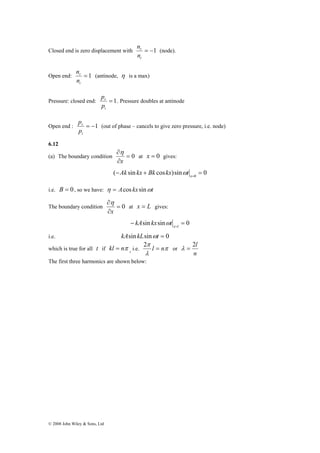
![η
0 l x n = 0 :
n =1:
η
0 l
6.13
The boundary condition for pressure continuity at x = 0 gives:
Aei ωt k x B ei ωt k x A e ω B e ω
Ae ω B e ω ω ω
© 2008 John Wiley & Sons, Ltd
0
( )
− + − = + 2
x
( )
0 2
( )
1
( )
1 [ 1 1 ] [ 2 2 ]
=
− −
=
i t k x i t k x
x
i.e. 1 1 2 2 A + B = A + B (6.13.1)
In acoustic wave, the pressure is given by: p = Zη& , so the continuity of particle velocity η& at
x = 0 gives:
( )
A e B e
2
− − +
2 0
( )
2
( )
1
1 0
( )
1
1 1 2 2
=
− −
=
=
+
x
i t k x i t k x
x
i t k x i t k x
Z
Z
i.e. ( ) ( ) 2 1 1 1 2 2 Z A − B = Z A − B (6.13.2)
At x = l , the continuity of pressure gives:
x l
i t k x
A ei t k x B ei t k x A e
− + − = ( )
[ ω 2 ω 2 ] ω 3
x l
=
−
=
3
( )
2
( )
2
A e−ik2l + B eik2l = A (6.13.3)
i.e. 2 2 3
The continuity of particle velocity gives:
l 3 x
n = 2 :
η
0 x
l 5 3l 5 l](https://image.slidesharecdn.com/136253314-physics-of-vibration-and-waves-solutions-pain-141001200006-phpapp01/85/physics-of-vibration-and-waves-solutions-pain-79-320.jpg)
![For a copper sphere of radius 1m, the time of decay of the field is approximately given by:
t = L2μσ = 12 ×1.26×10−6 ×5.8×107 ≈ 73[s] < 100[s]
7.17
f α t = r e− r in
Try solution ( , ) ( α )2
f t
f α t = r e− r in
f t
© 2008 John Wiley & Sons, Ltd
π
f t
∂
∂ (α , )
t
, we have:
dr
⎤
⎡
∂
r e r dr
2 2
r r
α α
( ) ( )
− −
= − +
r e 2
dr
2
2
r
α
( )
1 2
α
π
2 2
( )
2 2
( )
r
2 1
4
( 2 ) 1
( , )
α
α
α
π
π
α α
π
π
α
r
r
e
t dt
dt
e
dt
dt
r e
t t
−
−
−
−
=
−
=
⎥⎦
⎢⎣
∂
=
∂
∂
(A.7.17.1)
Try solution ( , ) ( α )2
π
f t
∂
∂ (α , )
x
, we have:
( , ) 2 3 α
f t = − −
∂
α r α e r
x
( )2
π
∂
so:
r e r e r r
( , ) 2 − r α 2 2 α
= − − −
r
α
2
( −
2 )
r r e
2
2
( )
= − −
2 2
2 2 ( )
3
( )
3
( )
3
2
2
r
2 1
4
2 (1 2 )
α
α
α
π
α
π
α
π
π
α
r
r
e
td dt
x
−
−
−
=
∂
∂
(A.7.17.2)
By comparing the above derivatives, A.7.17.1 and 2, we can find the solution
f α t = r e− r
( , ) ( α )2
π
satisfies the equation:
2
2
x
d f
f
t
∂
∂
=
∂
∂](https://image.slidesharecdn.com/136253314-physics-of-vibration-and-waves-solutions-pain-141001200006-phpapp01/85/physics-of-vibration-and-waves-solutions-pain-96-320.jpg)
![C W A W C
Currents in W into page. Field lines at A cancel. Those at C force wires together.
Reverse current in one wire. Field lines at A in same direction, force wires apart.
1 2 2
2
C W A Motion
−
a e −
= =
πε π
© 2008 John Wiley & Sons, Ltd
Fig Q.8.2.a
Field lines at C in same direction as those from current in wire –
in opposite direction at A . Motion to the right
Fig Q.8.2.b
8.3
The volume of a thin shell of thickness dr is given by: 4πr2dr , so the electrostatic
energy over the spherical volume from radius a to infinity is given
by: ∫+∞
a
E (4 r )dr
2
0 ε π , which equals mc2 , i.e.:
1 E r dr mc
∫ = +∞ ε π
2 2 2
0 (4 )
2
a
By substitution of 2
0 E = e 4πε r into the above equation, we have:
1 r dr mc
∫ = +∞ π
2 2
(4 )
2 0 (4 2 )
2
2
0
r
e
a
πε
ε
2 1
8
∫ = +∞
i.e. 2
2
0
dr mc
r
e
a
πε
2
8
e =
πε
i.e. 2
0
mc
a
Then, the value of radius a is given by:
1.41 10 [ ]
19 2
(1.6 ×
10 )
8 8.8 10 9.1 10 (3 10 )
8
15
12 31 8 2
2
0
m
mc
− −
≈ ×
× × × × × ×](https://image.slidesharecdn.com/136253314-physics-of-vibration-and-waves-solutions-pain-141001200006-phpapp01/85/physics-of-vibration-and-waves-solutions-pain-98-320.jpg)
![Another approach to the problem yields the value:
© 2008 John Wiley & Sons, Ltd
a = 2.82×10⁻¹⁵[m]
8.4
The magnitude of Poynting vector on the surface of the wire can be calculated by
deriving the electric and magnetic fields respectively.
The vector of magnetic field on the surface of the cylindrical wire points towards the
azimuthal direction, and its magnitude is given by Ampere’s Law:
H e e
θ θ θ π
r
H I
2
= =
where r is the radius of the wire’s cross circular section, and I is the current in the
wire.
Ohm’s Law, J =σE , shows the vector of electric field on the surface of the
cylindrical wire points towards the current’s direction, and its magnitude equals the
voltage drop per unit length, i.e.:
E = E e = V e = IR
e
z z l
z l z
where, l is the length of the wire, and the V is the voltage drop along the whole
length of the wire and is given by Ohm’s Law: V = IR, where R is the resistance of
the wire.
Hence, the Poynting vector on the surface of the wire points towards the axis of the
wire is given by:
z z z r S E H E e H e E H e θ θ θ = × = × = −
which shows the Poynting vector on the surface of the wire points towards the axis of
the wire, which corresponds to the flow of energy into the wire from surrounding
space. The product of its magnitude and the surface area of the wire is given by:
rl I R
× 2 = × 2 = π =
r
I
S rl E H rl IR z
l
2 2
2
π
π π θ
which is the rate of generation of heat in the wire.
8.5
By relating Poynting vector to magnetic energy, we first need to derive the magnitude
of Poynting vector in terms of magnetic field.
The electric field on the inner surface of the solenoid can be derived from the integral
format of Faraday’s Law:
Edl ∂
μ H
∫ ∫∂
= − dS
t
where S is the area of the solenoid’s cross section. E is the electric field on the
inner surface of the solenoid, and H is the magnetic field inside the solenoid.
For a long uniformly wound solenoid the electric field uniformly points towards
azimuthal direction, i.e. θ θ E = E e , and the magnetic field inside the solenoid](https://image.slidesharecdn.com/136253314-physics-of-vibration-and-waves-solutions-pain-141001200006-phpapp01/85/physics-of-vibration-and-waves-solutions-pain-99-320.jpg)
![Since the intensity in such a wave is given by:
S = 1 × × × × − × E ≈ × − E
= S = S S Vm
ε
= 0
= S = S S Am
Power 8 2
I = = Wm
×
E I
2 −
E = S = × ≈ Vm−
1 2 12 2 6
= ε + μ =ε = × − × = × −
© 2008 John Wiley & Sons, Ltd
2
I S c E 1 c E av = = ε = ε
0 max
2
0 2
we have:
2
max
3 108 8.8 10 12 1.327 10
2 3
max
2
2 2 1 2 1 2 1
27.45 [ ]
8 12
3 10 8.8 10
1 2
0
max
−
− ≈
× × ×
c
E
ε
2 2 1 2 2 1 2 1
7.3 10 [ ]
8 -7
3 10 4 10
1 2
0
max
0
max
≈ × − −
× × ×
c
H E
μ μ π
8.7
The average intensity of the beam and is given by:
1.53 10 [ ]
0.3
(2.5 10 ) 10
Energy
area pulse duration
area
3 2 4
−
− − = ×
× × ×
=
×
π
Using the result in Problem 8.6, the root mean square value of the electric field in
the wave is given by:
8
1.53 10 5 1
8 12
= = Vm
2.4 10 [ ]
3 10 8.8 10
0
− ≈ ×
× × ×
c
ε
8.8
Using the result of Problem 8.6, the amplitude of the electric field at the earth’s
surface is given by:
27.45 1 2 27.45 1350 1010[ 1]
0
and the amplitude of the associated magnetic field in the wave is given by:
7.3 10 2 1350 2.7[ 1]
H = × − × ≈ Am−
0
The radiation pressure of the sunlight upon the earth equals the sum of the electric
field energy density and the magnetic field energy density, i.e.
8.8 10 1010 8.98 10 [ ]
1
2
2
0 0
2
0 0
2
0 0 p E H E Pa rad
8.9
The total radiant energy loss per second of the sun is given by:
E S 4 r2 1350 4 (15 1010 )2 3.82 1026[J ] loss = × π = × π × × = ×
which is associated with a mass of:
3.82 10 9
4.2 10 [ ]
8 2
(3 10 )
26
m E c2 kg loss = ×
×
×
= =](https://image.slidesharecdn.com/136253314-physics-of-vibration-and-waves-solutions-pain-141001200006-phpapp01/85/physics-of-vibration-and-waves-solutions-pain-101-320.jpg)
![8.10
At a point 10km from the station, the Poynting vector is given by:
S P = × −
0 E = × S = × × − = V m
0 H = × − S = × − × × − = × − A m
© 2008 John Wiley & Sons, Ltd
1.6 10 [ ]
10
2 (10 10 )
2
4 2
3 2
5
W m
r
2 × × ×
= =
π π
Using the result in Problem 8.6, the amplitude of electric field is given by:
27.45 1 2 27.45 1.6 10 4 0.346[ ]
The amplitude of magnetic field is given by:
7.3 10 2 1 2 7.3 10 2 1.6 10 4 9.2 10 4[ ]
8.11
The surface current in the strip is given by:
I = Qv
where Q is surface charge per unit area on the strip and is given by: x Q =εE , and
v is the velocity of surface charges along the transmission line.
Since the surface charges change along the transmission line at the same speed as the
electromagnetic wave travels, i.e.
v = c = 1 , the surface current becomes:
με
ε
= = ε 1 =
x x I Qv E E
μ
με
Analysis in page 207 shows, for plane electromagnetic wave, y x μ H = ε E , so the
surface current is now given by:
μ
ε
y y I = H = H
ε
μ
On the other hand, the voltage across the two strips is given by:
x x V = E L = E
where L = 1 is the distance between the two strips.
Therefore the characteristic impedance of the transmission line is given by:
μ
ε
Z V
= = =
x
H
y
E
I
8.12
Write equation (8.6) in form:](https://image.slidesharecdn.com/136253314-physics-of-vibration-and-waves-solutions-pain-141001200006-phpapp01/85/physics-of-vibration-and-waves-solutions-pain-102-320.jpg)
![0.1
σ
(b) = = π
9 3 2
πνε ε π
σ
< π
π ε ε π
T H
© 2008 John Wiley & Sons, Ltd
4 6
0
36 10 3.6 10 10
2 10 10 50
2
× × = × − < −
× × ×
σ
ωε
r
which shows, at a frequency of 104MHz , the medium is a dielectric.
8.15
The Atlantic Ocean is a conductor when:
100
σ
= >
2 πνε ε
0
σ
ωε
r
4.3
i.e. 36 10 10[ ]
2 100 81
2 100
9
0
MHz
r
× × ≈
× ×
=
× ×
ν
Therefore the longest wavelength that could propagate under water is given by:
6
v c
= = = 10×10
λ ε λ
max max
ν
r
c 3 10
m
max 6 8
×
i.e. 3[ ]
10 10 81 10 10
6
r
≈
× ×
=
× ×
=
ε
λ
8.16
When a plane electromagnetic wave travelling in air with an impedance of air Z is
reflected normally from a plane conducting surface with an impedance of c Z , the
transmission coefficient of magnetic field is given by:
t
i
T = H
H H
Using the relations: t c t E = Z H , i air i E = Z H , and
= 2 c
, the above equation
Z
c air
E
t
i
Z Z
E
+
becomes:
air
Z
Z
E Z
= = = 2 2
H Z Z
c air
c
c air
air
c
t air
i c
t
i
Z
Z Z
Z
E Z
H
+
=
+
The impedance of a good conductor tends to zero, i.e. →0 c Z , so we have:
T ≈ 2 Z air
= 2
or H ≈ 2H
t i air
H Z
After reflection from the air-conductor interface, standing waves are formed in the air](https://image.slidesharecdn.com/136253314-physics-of-vibration-and-waves-solutions-pain-141001200006-phpapp01/85/physics-of-vibration-and-waves-solutions-pain-104-320.jpg)
![field Ex by a phase angle of φ = 45o , so we can write the electric field and magnetic
field in a conductor as:
(real part of ) 2
Z =
Z
copper copper 376.6 376.6 2
2
© 2008 John Wiley & Sons, Ltd
E E t x cosω 0 = and cos( ) 0 H = H ωt −φ y
so the average value of the Poynting vector is the integral of the Poynting vector
x y E H over one time period T divided by the time period, i.e.:
∫
0
=
1 cos ω cos( ω φ
)
cos 45 [ ]
∫
= −
0 0 0
1
∫
= − +
cos 1
2
E H
1
2
[cos(2 ) cos ]
2
1
2
0 0
0
0 0
E H
0 0
T E H Wm
T
t dt
T
E tH t dt
T
E H
T
S
T
T
T
av x y
= φ
= o
ω φ φ
Noting that the real part of impedance of the conductor is given by:
E
Z E c = φ =
(real part of ) cos 0
cos 45o
0
0
0
H
H
0 c E = H × Z o
i.e. 0
(real part of )
cos45
so we have:
S E H
0 0
H Z
=
= × ×
(real part of )[ ]
1
1
2
real part of cos45
1
2
0
2 cos45
cos45
2
2 2
0
H Z Wm
c
c
av
= ×
o
o
o
We know from analysis in page 216 that, at a frequency ν = 3000MHz , the value of
ωε σ for copper is 2.9×10⁻⁹ , hence, at of frequency of 1000MHz , the value of
ωε σ for copper is given by 2.9×10⁻⁹ 3 = 9.7×10⁻¹⁰ , and ≈ ≈ 1 r r μ ε . So, the real
part of impedance of the large copper sheet is given by:
9.7 10 8.2 10 [ ]
2
2
2
ωε
μ
= × × = × × × − 10 = × −
3 Ω
σ
r
ε
r
Noting that, at an air-conductor interface, the transmitted magnetic field in copper
copper H doubles the incident magnetic field 0 H , i.e. 0 H 2H copper = , the average](https://image.slidesharecdn.com/136253314-physics-of-vibration-and-waves-solutions-pain-141001200006-phpapp01/85/physics-of-vibration-and-waves-solutions-pain-106-320.jpg)
![power absorbed by the copper per square metre is the average value of transmitted
Poynting vector, which is given by:
⎛
1 I
1 1 2 ⎟ ⎟⎠
2ωε 0 = 8 8 8 0 = = r ∫
0
=
1 cos cos
=
∫
∫
E H
ω ω
= +
1
0 0 0
1
0
0 0
T E H E Wm
E H
© 2008 John Wiley & Sons, Ltd
S H Z
copper copper copper
1
1
H Z
(2 ) (real part of )
2
= ×
copper copper
H Z
2 (real part of )
8.2 10 1.16 10 [ ]
= ×
= ×⎛
2 1
376.6
(real part of )
376.6
2
(real part of )
2
3 7
2
2
0
2
2
2
W
E Z
copper
copper copper
⎞
⎞
− − × = × × ⎟⎠
= ×⎛
⎜⎝
× ⎟⎠
⎜⎝
= ×
8.18
Analysis in page 222 and 223 shows that when an electromagnetic wave is reflected
normally from a conducting surface its reflection coefficient r I is given by:
ωε 0 = 1− 2 2 r I
σ
Noting that = 1 r ε
, the fractional loss of energy is given by:
ωε
σ
ωε ε
σ
ωε
σ
σ
⎞
⎜ ⎜⎝
− = − − r
8.19
Following the discussion of solution to problem 8.17, we can also find the average
value of Poynting vector in air.
The electric and magnetic field of plane wave in air have the same phase, so the
Poynting vector in air is given by:
S = E H = E cos ω t × H cos ω t = E H cos
2ω
t air x y 0 0 0 0 and its average value is given by:
1.33 10 [ ]
1
2 376.6
1
2 376.6
1
2
2
[1 cos(2 )]
2
1
3 1
2
0
0 0
0 0
= × − −
×
= = = × =
T
t dt
T
E tH tdt
T
E H
T
S
T
T
T
air x y
ω](https://image.slidesharecdn.com/136253314-physics-of-vibration-and-waves-solutions-pain-141001200006-phpapp01/85/physics-of-vibration-and-waves-solutions-pain-107-320.jpg)
![So, the ratio of transmitted Poynting vector in copper to the incident Poynting vector
in air is given by:
⎞
⎛
− − − − −
E H Ae e A e e e
1
1
⎞
⎛
real part of 1 2 2
S = ⎛ E H A e kz Wm
av x y ωμ
(average electric energy density) 1ε ε
T kz kz T kz
= ∫ = ∫ ω
2 2 2 2
© 2008 John Wiley & Sons, Ltd
−
= ×
1.16 10 −
5
7
3
8.81 10
×
1.33 10
−
×
=
copper
S
air
S
which equals the fractional loss of energy r I given by:
ωε
= 8 = 8×9.7×10−10 = 8.81×10⁻⁵
σ
r I
8.20
x E and y H are in complex expression, we have:
σ
kz i t kz kz i t kz i
ω ω π
2 4
1 2
2
( ) 4
1 2
1
* ( )
2
2
2
π
σ
⎞
ωμ
ωμ
kz i
x y
−
⎛
A e e
⎟ ⎟⎠
⎜ ⎜⎝
=
⎟ ⎟⎠
⎜ ⎜⎝
=
So, the average value of the Poynting vector in the conductor is given by:
[ ]
1
2 2
2
1 2
⎞
* 2 − −
⎟ ⎟⎠
⎜ ⎜⎝
= ⎟⎠
⎜⎝
σ
The mean value of the electric field vector, x E , is a constant value, which contributes
to the same electric energy density at the same amount of time, i.e.:
1 1
= = ∫T
2 2
x x E dt
T
E
0
2
2
i.e.
1 cos 1 1 cos2 2 2
2 2
0
2 2
0
x
t dt A e
T
tdt A e
T
E A e
−
+
− ω
− =
2
or: kz
x E = Ae−
2
Noting that:
2 1
σ
⎞
⎛
av kz
k A e
2 2
ωμ
⎛
ωμσ σ
⎞
⎞
∂
= − ⎛
A e
2 2
2
2
1 2 1 2
2
2
1 2
2
2
2 2
x
kz
kz
A e E
S
z
σ
σ
ωμ
= − = −
⎟ ⎟⎠
⎜ ⎜⎝
⎟⎠
⎜⎝
⎟ ⎟⎠
⎜ ⎜⎝
= − ×
∂
−
−
−](https://image.slidesharecdn.com/136253314-physics-of-vibration-and-waves-solutions-pain-141001200006-phpapp01/85/physics-of-vibration-and-waves-solutions-pain-108-320.jpg)
![The loss of intensity is given by:
2
⎞
⎛
+
⎞
⎛
+
⎞
⎛
I Z E Z
2 Z
Z
2
1 2
n
=
i t
I
t 2 (1 )
© 2008 John Wiley & Sons, Ltd
1 2 1 loss t t I = − I I
where t1 I is the transmittivity from air to glass and t 2 I is the transmittivity from
glass to air. Following the discussion in problem 8.21, we have:
2 1
2 2
0 0
2
0
0
0
2
4
1 1
1
t
d
d
d
d
t i
n
Z Z Z n n
Z Z
Z
Z E
+
= ⎟ ⎟⎠
⎜ ⎜⎝
= ⎟ ⎟⎠
⎜ ⎜⎝
= ⎟ ⎟⎠
⎜ ⎜⎝
+
= =
So we have:
1 2 1 0.962 7.84%
1 = − = − = loss t I I
8.24
Noting that 1 μ ε λω 2π 0 0 c = = , the radiating power can be written as:
2
0
q x
q
ω
x I
2
μ ε
0
ω
πε λ ω
π μ
= × 0
⎛
0
2
2 2 0 0 0
x
P dE
0
2
0
2 2
2 2
2
0
2
0
2
3
0
2
0
2 4
2
3
12
4
12
1
2
12
x I
c c
c
dt
⎞
⎟⎠
⎜⎝
=
⋅
=
= =
ε λ
π ω
ω
πε
πε
2 2
R π μ x x
= ⎛ ⎟⎠
= ⎛
i.e. 787 [ ]
3
0 0
⎟⎠
Ω 2
0
0
⎞
⎜⎝
⎞
⎜⎝
ε λ λ
By substitution of given parameters, the wavelength is given by:
m x m
600[ ] 30[ ]
8
3 ×
10
5 10
5 0
ν
c
= >> =
×
= =
λ
So the radiation resistance and the radiated power are given by:
1.97[ ]
2 2
R x
787 787 30
= ×⎛ ⎟⎠
0 = Ω ⎟⎠
600
⎞
⎜⎝
⎞
= ×⎛
⎜⎝
λ
1 2 1
2
0 P = RI = × × ≈ W
1.97 20 400[ ]
2
2](https://image.slidesharecdn.com/136253314-physics-of-vibration-and-waves-solutions-pain-141001200006-phpapp01/85/physics-of-vibration-and-waves-solutions-pain-110-320.jpg)
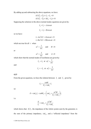
![SOLUTIONS TO CHAPTER 9
9.1
∂
+
∂
Substituting the expression of z into 2
∂ ω − +
k 2 =ω2 c2 = k + k , we have:
z = A{ei ωt− k1x+k2 y − ei ωt− k1x−k2 y } = A [ei ωt−k1x (e−ik2 y − eik2 y )] = −2iA sin(k y)ei ωt−k1x
Therefore, the real part of z is given by:
© 2008 John Wiley & Sons, Ltd
2
2
2
y
z
x
z
∂
∂
, we have:
k k Ae k k z
∂
+
y
z
x
z ( ) i t k x k y ( 2 )
2
2
1
2 [ ( )]
2
2
2 1
2
2
2
= − + 1 2 = − +
∂
∂
Noting that 2
2
2
1
z
2 ω
z
∂
+
y c
∂
x
z
2
2
2
2
2
= −
∂
∂
2
1
∂
Substituting the expression of z into 2
2
t
z
c ∂
, we have:
2
1 2 1 = −ω ω = −ω
∂
z
c
Ae
z
t c
c
t k x k y
2
[ ( )]
2
2
2
2
2
∂ − +
So we have:
2
2
2 1
z
2 2
2
2
t
z
∂
+
y c
∂
x
z
∂
∂
=
∂
∂
9.2
Boundary condition z = 0 at y = 0 gives:
Aei ωt−k1x + A ei ( ωt−k1x ) = 0
i.e. A = −A
1 2 2
( )
1
so the expression of z can be written as:
( )
1 2
( )
1
[ ( )] [ ( )]
1
2 sin sin( ) 1 2 1z A k y t k x real = + ω −
Using the above expression, boundary condition z = 0 at y = b gives:
z = − iA k bei ωt−k1x =
2 sin ( ) 0
1 2
which is true for any t and x , provided: sin 0 2 k b = , i.e.
k nπ
= 2 .
b](https://image.slidesharecdn.com/136253314-physics-of-vibration-and-waves-solutions-pain-141001200006-phpapp01/85/physics-of-vibration-and-waves-solutions-pain-111-320.jpg)
![9.3
As an analogy to discussion in text page 242, electric field z E between these two planes is the
superposition of the incident and reflected waves, which can be written as:
0 ( ) i k x k y t i k x k y t ik x ik x i k y t
z
+ = ⎛
μ
© 2008 John Wiley & Sons, Ltd
[( ) ]
E E e x y E e x y + −ω − + −ω = +
2
[( ) ]
1
i k x k y t i k x k y t
z
where k k cosθ x = and k k sinθ y =
Boundary condition = 0 z E at x = 0 gives:
1 2 + = E E ei ky y− t ω
( ) 0 ( )
which is true for any t and y if 1 2 0 E = −E = E , so we have:
( )
0
[( ) ]
0
[( ) ]
E E e x y E e x y E e x e x e y + −ω − + −ω − −ω = − = −
Using the above equation, boundary condition = 0 z E at x = a gives:
( ) 0 ( )
0 = − = ik a −ik a i k y− t
z
E E e x e x e y ω
i.e. sin k ae i ( k y y− ω
t
) = 0 x
which is true for any t and y if sin k a = 0 x , i.e. k n a x = π .
By substitution of the expressions for c λ
and g λ
1 1
c g λ λ
+ , we have:
into 2 2
20
2
= = ⎛
2
2
2 2 2 2
2
2 2
1
ω
⎞
⎛
+ ⎟⎠
2 2 (2 ) (2 ) 2
1 1
⎞
π λ
λ λ π π π π
= ⎟⎠
⎜⎝
+
= ⎟ ⎟⎠
⎜ ⎜⎝
⎞
⎜⎝
c
kx ky kx ky k
c g
9.4
Electric field components in x, y, z directions in problem 9.3 are given by:
0 ( ) ik x ik x i k y t
E = E = 0 and E = E e − e − e ( y −ω
)
x x x y z
By substitution of these values into equation 8.1, we have:
− −
x x y
ik x ik x i k y t
( )
( )
∂
E ik E e e e
x
0
( )
0
( )
∂
=
y z x
ik x ik x i k y t
x z y
x x y
∂
∂
H
t
E ik E e e e
y
H
t
ω
ω
μ
− −
= − +
∂
= −
∂
−
= −
∂
∂
−
which yields:](https://image.slidesharecdn.com/136253314-physics-of-vibration-and-waves-solutions-pain-141001200006-phpapp01/85/physics-of-vibration-and-waves-solutions-pain-112-320.jpg)
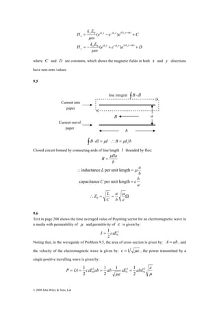
![i ω t − k x + k y i ω t − − k x + k y i ω t − k x − k y i ω
t − − k x −
k y
z = A { e − e } + A {
e −
e
1 2 1 2 1 2 1 2
i ω t − k y i ω
t +
k y
Ai k xe A i k xe
2 sin 2 sin
= − +
− +
ω ω
i k x Ae A e
= − −
k nπ 1
1 = , where 1,2,3,L 1 n = .
© 2008 John Wiley & Sons, Ltd
1 1
a b
ω =πc +
min 2 2
9.10
The dispersion relation of the waves of Problem 9.7 – 9.9 is given by:
⎞
⎟ ⎟⎠
⎛
k c m x ω π
⎜ ⎜⎝
2
2
n
= − + 2
2
2 2 2 2
b
a
The differentiation of this equation gives:
2 = 2
k dkx x 2
ωdω
c
d
k x x
i.e. c2
dk
=
ω ω
or v v c2 p g =
9.11
Using boundary condition z = 0 at x = 0 in the displacement equation gives:
A + A ei ωt−k2 y + A + A ei ωt+k2 y =
( ) ( ) ( ) 0
2 3
( )
1 4
which is true for any t and y if:
1 4 A = −A and 2 3 A = −A
so we have:
2 2
i t k y i t k y
( )
2 sin [ ]
2
( )
1 1
( )
2 1
( )
1 1
[ ( )] [ ( )]
2
[ ( )] [ ( )]
1
2 2
(9.11.1)
Using boundary condition z = 0 at y = 0 in equation (9.11.1) gives:
2 sin ( ) 0 1 1 2 − i k x A − A eiωt =
which is true for any t and x if:
1 2 A = A
Therefore, equation (9.11.1) becomes:
z A k x k yeiωt
1 1 2 = −4 sin sin
and the real part of z is given by:
z A k x k y t real 4 sin sin cosω 1 1 2 = − (9.11.2)
Using boundary condition z = 0 at x = a in equation (9.11.2) gives:
sin 0 1 k a = , i.e.
a](https://image.slidesharecdn.com/136253314-physics-of-vibration-and-waves-solutions-pain-141001200006-phpapp01/85/physics-of-vibration-and-waves-solutions-pain-116-320.jpg)
![Using boundary condition z = 0 at y = b in equation (9.11.2) gives:
sin 0 2 k b = , i.e.
k n π 2
2 = , where 1,2,3,L 2 n = .
e−hν kTN = e−hν kTΣN = N e− ν + e− ν + e− ν +L+ e− + ν
=Σ =Σ = Σ
E E N nh h N n
ν ν ν ν ν
= − + − + − + + −
Ee−hν kT = hνN e− hν kT + e− hν kT + e− hν kT +L+ ne− n+ hν kT
ν ν ν ν ν ν
E Ee h N e e e e ne
ν ν ν ν ν
h N e e e e ne
lim[1 ]
= + + + + −
ν
⎛
h ν
N e e
lim 1
0
−
h kT
h kT
h kT
N h e
e
E
ν
= = − −
© 2008 John Wiley & Sons, Ltd
b
9.12
Multiplying the equation of geometric progression series by e−hν kT on both sides gives:
h kT h kT h kT n h kT
[ 2 3 ( 1) ]
0
n
n
so we have:
0
N − e − h ν kT N = N [1 − lime − ( n + 1)
h ν
kT ] =
N
0 n
→∞
i.e.
N N − − ν
e h kT
=
1
0
The total energy over all the n energy states is given by:
n
n
n
n
ν ν
h kT h kT h kT nh kT
( 2 2 3 3 )
0
n
n
h N e e e L
ne
Multiplying the above equation by e−hν kT on both sides gives:
[ 2 2 3 3 4 ( 1) ]
0
so we have:
−
−
1
h kT
h kT
nh ν
kT
h kT nh kT
n
h kT
h kT h kT n h kT nh kT
n
h kT
h kT h kT h kT nh kT n h kT
n
h kT
e
h N e
e
n
e
ν
ν
ν ν
ν
ν
ν
−
−
−
→∞
−
− − − − −
→∞
−
− − − − − +
→∞
−
−
=
⎞
⎟ ⎟⎠
⎜ ⎜⎝
−
−
=
− = + + + + −
1
1
lim[ ]
0
2 ( 1)
0
2 3 ( 1)
0
L
L
−
h kT
e
ν ν
E N h e ν
i.e. 0 (1 −
−
h kT )2
=
Hence, the average energy per oscillator is given by:
1 1
0 2
(1 )
1
0
−
=
−
=
−
−
N
−
−
h kT h kT
h kT
e
h
e
h e
e
N
ν ν
ν
ν
ν
ν
ν
ν
ε
By expanding the denominator of the above equation for hν << kT , we have:](https://image.slidesharecdn.com/136253314-physics-of-vibration-and-waves-solutions-pain-141001200006-phpapp01/85/physics-of-vibration-and-waves-solutions-pain-117-320.jpg)
![2 ( ) 8
1 ( ) 1
( ) 1
π
X x 2
© 2008 John Wiley & Sons, Ltd
kT
h h
ν
≈ =
h kT
ν
h kT h kT
+ + + −
=
ν
ν ν
ε
[1 ( )2 2 L] 1
which is the classical expression of Rayleigh-Jeans for an oscillator with two degrees of freedom.
Alternative derivation for E and ε :
E = Nε = Nnhν where
ν ν
nh e
Σ
Σ
∞
=
−
∞
=
−
=
0
0
( )
n
nh kT
n
nh kT
e
nh
ν
ν
ν
∂
log 1
kT e
h ν
kT
h kT
n
h kT
nh kT
h e
−
e
e
kT
nh
ν
ν
ν
ν
−
− −
∞
=
−
−
−
=
∂ −
= −
∂
∂
∴ = − Σ
1
1
( )
log
( )
1
0
1
h kT
2
ν ν
E Nnh ν N h e−
ν
0
(1 e
h kT )
−
−
∴ = =
and
−1
nh h ν
ν
ε ν
= = e−h kT
9.13
One solution of this Schrodinger’s time-independent equation can be written as:
ψ = X (x)Y( y)Z(z)
Substituting this expression into the Schrodinger’s equation and dividing ψ on both sides of the
equation, we have:
E
h
m
Z z
z
Y y
y Z z
X x
x Y y
2
2
2
2
2
2
( )
( )
( )
= −
∂
∂
+
∂
∂
+
∂
∂
which yields:
X x
( ) ( ) 0
Y y
x
( ) ( ) 0
Z z
y
( ) ( ) 0
2
2
2
2
2
2
+ =
∂
∂
+ =
∂
∂
+ =
∂
∂
E Z z
z
E Y y
y
E X x
x
z
8π 2
E E E m x y z 2
where x y z E ,E ,E are constants and satisfy: E
h
+ + =
By solving the above three equations, we have:](https://image.slidesharecdn.com/136253314-physics-of-vibration-and-waves-solutions-pain-141001200006-phpapp01/85/physics-of-vibration-and-waves-solutions-pain-118-320.jpg)
![5 4
15
a k π
8
c h
=
x ch
© 2008 John Wiley & Sons, Ltd
E d kTx
8 ( )
∞ ∞
∫ ∫
0 4
kT x
8 ( )
kT
8 ( )
( ) ( 1)
π π
= ×
ch
( ) 15
4
5 4
k
3 3
4
3
4
0 3
4 3
5
0
8
15
( ) ( 1)
T
c h
dx
ch e
d ch
xkT
ch e
x
x
π
π
π
λ λ
=
−
=
−
=
∫
∞
i.e.
4
∫ E d = aT ∞ λ λ
0
where 3 3
9.16
Using the expression of λ E in Problem 9.15, the wavelength m λ at which λ E is maximum
should satisfy the equation:
d
= 0 λ E
dx
which yields:
0
5
x
( 1)
=
ex −
d
dx
x x
e
4 5
x e e x
5 ( 1)
− −
x
i.e. 0
( 1)
2
=
−
⎛ − x ex
i.e. 1
1 5
⎟⎠
= ⎞
⎜⎝
where
kT
λ
=
9.17
The most sensitive wavelength to the human eye can be given by substituting the sun’s
temperature T = 6000[K] into equation ch kT m λ = 5 , i.e.:
4.7 10 [ ]
8 34
3 × 10 × 6.63 ×
10
5 1.38 10 6000
ch
5
7
23
m
kT
m
−
−
−
≈ ×
× × ×
λ = =
which is in the green region of the visible spectrum.](https://image.slidesharecdn.com/136253314-physics-of-vibration-and-waves-solutions-pain-141001200006-phpapp01/85/physics-of-vibration-and-waves-solutions-pain-121-320.jpg)
![9.18
Substituting the tungsten’s temperature T = 2000[K] into equation ch kT m λ = 5 , i.e.:
S E dE m Ed E L
© 2008 John Wiley & Sons, Ltd
14 10 [ ]
8 34
3 × 10 × 6.63 ×
10
5 1.38 10 2000
ch
5
7
23
m
kT
m
−
−
−
≈ ×
× × ×
λ = =
which is well into infrared.
9.19
As an analogy to the derivation of number of points in ν state shown in text page 250, 251, the
number of points in k space between k and k + dk is given by:
(volume of spherical shell)
8
2 3
8
πk dk L
4
volume of cell
1
⎞
⎟⎠
= ⋅⎛
⎜⎝
π
Noting that for each value of k there are two allowed states, the total number of states in k
space between k and k + dk is given by:
2 3
8
P k πk dk L
( ) = 2 ⋅ 4 ⋅⎛
⎞
⎟⎠
⎜⎝
π
From E = (h2 2m*)k 2 , we have k = (2m* h2 )E . By substitution into the above equation,
we get the number of states S(E)dE in the energy interval dE given by:
( ) 2 4 (2 )
3 * 2 3 2
h
⎞
dE L m E dE
3 * 2 3 2
L m E
(2 )
E
(2 )
2
2
* 2 3 2 3
2
2
8
π π
π
π
h h
= =
⎟⎠
⎜⎝= ⋅ ⎛
Provided m ≈ m* and A = L3 , we have:
3 2
S E = A ⎛
2
m E
⎟⎠
( ) 2
2 2
⎞
⎜⎝
π h
Since Fermi energy level satisfies the equation:
∫ Ef S ( E )
dE = N 0
By substitution of the expression of S(E) , we have:
⎟⎠
Ef A m ⎞
EdE = N ⎛ ∫0
⎜⎝
3 2
2
2 2
2π h
i.e.](https://image.slidesharecdn.com/136253314-physics-of-vibration-and-waves-solutions-pain-141001200006-phpapp01/85/physics-of-vibration-and-waves-solutions-pain-122-320.jpg)
![Overall, the Fourier series is given by:
1
= +Σ +Σ∞ ∞
y a a nx b nx n n
0
π
h
⎛
x x x xL a =
4 h sin x cos 2
nx dx n
h x nxdx
4 π
sin cos2
π
π
∫
h n x n x dx
2 [sin(1 2 ) sin(1 2 ) ]
=
= + + −
π
a h ,
1 ⋅
y a a nx n
© 2008 John Wiley & Sons, Ltd
⎞
⎟⎠
⎜⎝
cos4 2
⋅
−
cos2 2
⋅
−
sin 2
⋅
−
⋅
= +
cos6
5 7
3 5
1 3
1 2
1
cos sin
2
1 1
π
10.4
Such a wave form is a even function with a period of π . Hence, there are only
constant term and cosine terms.
The constant term is given by:
a 1 π hsin xdx 2h
2
π π
1
0 0 = ∫ =
which doubles the constant shown in Problem 10.3
The coefficient of cosine term is given by:
2
0
2
0
2
0
2
0
⎡ −
cos(1 2 )
cos(1 2 ) 1
1 2
2 1
1 2
π
π
π
π
π
π
⎤
⎥⎦
⎢⎣
−
+ +
+
= −
∫
∫
n x
n
n x
n
h
which gives:
2
1 3
= −
π
a h 2
,
2 ⋅
3 5
= −
π
a h 2
, …
3 ⋅
5 7
= −
π
Therefore the Fourier series is given by:
⎞
⎟⎠
1
+ = Σ∞
π
h
⎛
x x xL ⎜⎝
cos4 2
⋅
−
cos2 2
⋅
−
1 2
⋅
= −
cos6
5 7
3 5
1 3
cos 2
2
1
0
π
π
Compared with Problem 10.3, the modulating ripple of the first harmonic h sin x
2
disappears.
10.5
f (x) is even function in the interval ±π , so its Fourier series has a constant term
given by:
1 2
( ) 1
2 3
1
2
2
2
0
π
π π
π
π
π
π
= ∫ = ∫ = − −
a f x dx x dx](https://image.slidesharecdn.com/136253314-physics-of-vibration-and-waves-solutions-pain-141001200006-phpapp01/85/physics-of-vibration-and-waves-solutions-pain-126-320.jpg)
![The coefficient of cosine term is given by:
a 2 f ( x π
)cos 2
nx dx
2 π cos 2 π
sin
∫ ∫
= =
π π
2 sin π π sin 4 π
cos
∫ 2
∫
0
π π
2 0 0 2 2
( ) 1 nx
= ∫ = ⋅ =
© 2008 John Wiley & Sons, Ltd
0 2 0
0
2
0
2
0
2
4 cos cos 4 cos ( 1) 4
n
n
n
x nx nxdx
n
xd nx
n
x nx nxdx
n
x d nx
n
x nxdx
n
n
− = = ⎥⎦ ⎤
⎢⎣ ⎡
= −
= ⎥⎦ ⎤
⎢⎣ ⎡
= −
2
=
∫
∫
π
π
π
π
π π
π
Therefore the Fourier series is given by:
cos 2
π
1
( 1) 4 cos
0 Σ Σ∞ ∞
= + = + −
1
2
2
1
3
2
2
n
f x a a nx n
n π
π
10.6
The square wave function of unit height f (x) has a constant value of 1 over its first
half period [0,π ], so we have:
f (π 2) = 1
By substitution into its Fourier series, we have:
1
sin 5
5
⎟⎠
( 2 ) ≈ 4 ⎛ sin + 1
sin 3
+
1
⎞
= 2
3
2
2
⎜⎝
π π π
π
f π
i.e.
1
7 4
1
5
1 1
3
π
− + − =
10.7
It is obvious that the pulse train satisfies f (t) = f (−t) , i.e. it is an even function. The
cosine coefficients of its Fourier series are given by:
nx
nx
τ n
τ
π
π
π π
τ
π
T n T
n
T
T
dx
T
T
an
sin 2 2 sin 2
2
4 cos 2 4
0
0
10.8
As τ becomes very small, τ
2 π π
sin τ
→ 2 n
, so we have:
T
n
T
= 2 sin 2 ≈ 2 ⋅ 2 = 4
T
n
n T
n
n T
an
τ
τ
π
π
τ
π
π
We can see as τ →0 , →0 n a , which shows as the energy representation in time](https://image.slidesharecdn.com/136253314-physics-of-vibration-and-waves-solutions-pain-141001200006-phpapp01/85/physics-of-vibration-and-waves-solutions-pain-127-320.jpg)
![+∞ − ′
−∞
F f t e dt
= ′
© 2008 John Wiley & Sons, Ltd
( ) ( )
2 2 ( )
2 0
f e dt
2 π ( ν ν
)
i t
0
( )
sin[ π ( ν ν ) τ
]
π ν ν τ
τ
π ν ν
π ν ν
ν
π ν ν τ π ν ν τ
τ
τ
π ν ν
τ π ν ν
τ
πν
( )
[ 2 ( ) ]
2 ( )
0
0
0
2 ( ) 2 2 ( ) 2
0
0
2
2 ( )
2 0
0
0
2
0 0
0
−
−
=
−
− −
=
− − ′
− −
=
= ′ ′
− − −
+
−
− − ′
+ − − ′
−
∫
∫
∫
f
e e
i
f
e d i t
i
f
i i
i t
i t
which shows the relative energy distribution in the spectrum given by:
π ( ) ( ) sin [ ( ν ν ) τ
]
2
0
0
2
2
0
2
[ π ( ν ν ) τ
]
ν τ
−
−
F = f
follows the intensity distribution curve in a single slit diffraction pattern given by:
I = I d
sin ( sin )
π θ λ
π θ λ
d
2
2
0 ( sin )
10.12
The energy spectrum has a maximum when:
1
sin [ π ( ν ν ) τ
]
2
max 0
[ ( ) ]
max 0
2
=
−
−
π ν ν τ
i.e. ( ) 0 min 0 π ν −ν τ = or min 0 ν =ν
The frequencies for the minima of the energy spectrum are given by:
0
sin [ π ( ν ν τ
( ) ( ) ) ] min 0
2
[ ( ) ]
min 0
2
2
min 0 =
−
−
=
π ν ν τ
F ν f τ
i.e. π (ν n −ν )τ = nπ min 0 or
ν n −ν = n min 0
τ
where n = −∞,L,−3,−2,−1,1,2,3,L,+∞
Hence, the total width of the first maximum of the energy spectrum is given by:
2 ν ν ν 1 2
1
min Δ = + − − = or
τ
min
Δν = 1
τ
Using the differentiation of the relation
ν = c :
λ
c
Δν = Δ 2
λ
λ
we have](https://image.slidesharecdn.com/136253314-physics-of-vibration-and-waves-solutions-pain-141001200006-phpapp01/85/physics-of-vibration-and-waves-solutions-pain-129-320.jpg)
![E = E e−ω0t Q = E e− where Q = t 0 ω
(ν ) ( ) 2πν πν 0 τ πν π ν 0 ν τ
© 2008 John Wiley & Sons, Ltd
2 Δ = c or
τ
λ
λ
1
λ
λ
τ
Δ
=
2
c
which is the coherence length l of Problem 10.11.
10.13
Use the relation ν
20
λ
Δλ = Δ
c
, we have:
(6.936 10 ) 4 17
10 1.6 10 [ ]
×
3 10
8
7 2
− m
−
× ≈ ×
×
Δλ =
Then, using the result in Problem 10.12, the coherence length is given by:
2 7 20
(6.936 ×
10 ) 4
λ
l = × m
3 10 [ ]
= −
1.6 10
17
×
=
Δ
−
λ
10.14
Referring to pages 46 and 47 of the text, and in particular to the example of the
radiating atom, we see that the energy of the damped simple harmonic motion:
1
0 0
, the period for which the atom radiates
0 before cut off at 0 ω
ω
e−1 .
The length of the wave train radiated by the atom is l = ct where c is the velocity
of light and l is the coherence length which contains Q radians.
Since the coherence length is finite the radiation cannot be represented by a single
angular frequency but by a bandwidth Δω centred about .
Now =ω Δω 0 Q so ω = =1 Δω 0 Q t . Writing t = Δt we have ΔωΔt =1 or
ΔνΔt =1 2π .
The bandwidth effect on the spectral line is increased in a gas of radiating atoms at
temperature T . Collisions between the atoms shorten the coherence length and the
Doppler effect from atomic thermal velocities adds to Δν .
10.15
The Fourier transform of f (t) gives:
∫ ∫ ∫+∞
+∞ − −
−∞
−∞
+∞ − −
−∞
F = f t e−i tdt = f ei te t e i tdt = f e[i2 ( ) 1 ]tdt
0
2 2
0
Noting that t ≥ 0 for f (t) , we have:](https://image.slidesharecdn.com/136253314-physics-of-vibration-and-waves-solutions-pain-141001200006-phpapp01/85/physics-of-vibration-and-waves-solutions-pain-130-320.jpg)
![F f
= f f
P F
2
0 ( )
P F r av =
r m s
2
f = F r and
2 0
0 2m
© 2008 John Wiley & Sons, Ltd
i π ν ν τ
t
F f e dt
{ }
( )
2 ( ) 1
π ν ν τ
2 ( ) 1 1 2 ( )
0
0
0
0
0
[ 2 ( ) 1 ]
0
0
0
[ 2 ( ) 1 ]
0
0
0
π ν ν τ τ π ν ν
ν
π ν ν τ
+ −
=
− −
= −
− −
=
=
− − +∞
+∞ − − ∫
i
f
i
f
e
i
f
i t
Hence, the energy distribution of frequencies in the region 0 ν −ν is given by:
2
0
2
2
0
2
0
2
2
0
2
0
2
2
0
2 0
f
1 2 ( ) (1 ) [2 ( )] (1 ) ( )
( )
τ π ν ν τ π ν ν τ ω ω
ν
+ −
=
+ −
= =
+ −
r
i
10.16
In the text of Chapter 3, the resonance power curve is given by the expression:
2
0
F r
F r
= = =
av + −
2 2[ ( ) ]
cos
2 2
2 2
2
0
2
0
ω ω
φ
r m s
Z
Z
m m
In the vicinity of = s m 0 ω
, we have 0 ω
ω ≈ , so the above equation becomes:
2
f F
2
0
2
2
0
2
0
F r
2 2
2
0
2 2
r m
2[ ( ) ] 2[ ( ) ] (1 ) ( )
ν
ω ω ω ω τ + ω −
ω
=
+ −
=
+ −
≈
where 2
τ = m
r
The frequency at half the maximum value of 2 F(ν ) is given by:
ν o F f = f
( )
2
(1 ) ( )
( )
2
2
0
2
2
2 0 τ
τ + ω −
ω
=
i.e. ω ω 1τ 0 − = ±
so the frequency width at half maximum is given by:
Δω = 2 τ or Δν = 1 πτ
In Problem 10.12 the spectrum width is given by:
Δν ′ = 1τ
so we have the relation between the two respectively defined frequency spectrum
widths given by:
ν
π
ν
Δ ′
Δ =](https://image.slidesharecdn.com/136253314-physics-of-vibration-and-waves-solutions-pain-141001200006-phpapp01/85/physics-of-vibration-and-waves-solutions-pain-131-320.jpg)
![20
λ
Noting that Δλ = Δ
ν
c
© 2008 John Wiley & Sons, Ltd
20
λ
Δλ′ = Δ ′
and ν
c
, we have:
λ
π
λ
Δ ′
Δ =
where Δλ and Δλ′ are the wavelength spectrum widths defined here and in
Problem 10.12, respectively.
If the spectrum line has a value Δλ = 3×10⁻⁹m in Problem 10.12, the coherence
length is given by:
2 7 20
(5.46 10 ) 6
32 10 [ ]
×
3 10
9
20
λ
λ
l − m
−
−
≈ ×
× ×
=
Δ
=
Δ ′
=
λπ π
λ
10.17
The double slit function (upper figure) and its self convolution (lower figure) are
shown below:
Fig. A.10.17
10.18
The convolution of the two functions is shown in Fig. A.10.18.1.
Fig. A.10.18.1
τ
d
τ
2τ d −τ 2τ d −τ 2τ
⊗ =
d d d d](https://image.slidesharecdn.com/136253314-physics-of-vibration-and-waves-solutions-pain-141001200006-phpapp01/85/physics-of-vibration-and-waves-solutions-pain-132-320.jpg)
![The convolution O(R) in the region [0,2r] is sketched below:
© 2008 John Wiley & Sons, Ltd
O(R)
0 2r R
Fig. A.10.19
πr2](https://image.slidesharecdn.com/136253314-physics-of-vibration-and-waves-solutions-pain-141001200006-phpapp01/85/physics-of-vibration-and-waves-solutions-pain-135-320.jpg)
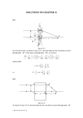
![is the same as through path A′B′ , so we have:
λ
sin
x = .
′
y ′
=
l
© 2008 John Wiley & Sons, Ltd
z
c
= ( ) 2
n d n α
r d
0 0 +
c
c
−
which yields:
z =αr2d
i.e.
= 1
d
f
2α
11.3
Choosing the distance PF = λ 2 then, for the path difference BF − BF′ , the phase
difference is π radians.
Similarly for the path difference AF′ − AF the phase difference is π radians.
Thus for the path difference AF′ − BF′ the phase difference is 2π radians and the
resulting amplitude of the secondary waves is zero.
Writing F′F = x 2 , we then have in the triangle F′FP :
x θ = , so the width of
2
sin
2
λ
the focal spot is
θ
11.4
If a man’s near point is 40cm from his eye, his eye has a range of accommodation of:
2.5[dioptres]
1 =
0.4
Noting that a healthy eye has a range of accommodation of 4 dioptres, he needs
spectacles of power:
P = 4 − 2.5 = 1.5[dioptres]
If anther man is unable to focus at distance greater than 2m, his eye’s minimum
accommodation is:
0.5[dioptres]
1 =
2
Therefore, he needs diverging spectacles with a power of -0.5 dioptres for clear image
of infinite distance.
11.5
Noting that
l
y
, we have the transverse magnification given by:
′
= . The
M l T
l
angular magnification is given by:
M y l d
0
l
= = =
γ
y d
0
β
α . Using the thin lens power](https://image.slidesharecdn.com/136253314-physics-of-vibration-and-waves-solutions-pain-141001200006-phpapp01/85/physics-of-vibration-and-waves-solutions-pain-137-320.jpg)
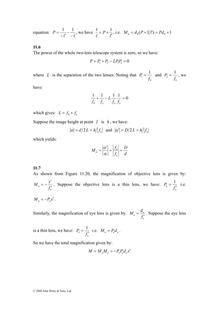
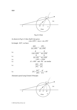
![IP k c d n OP n R
P n n and 1 1.5 0
1 = −
α α α
⎡
′
2
⎡
=
⎤
1 0
© 2008 John Wiley & Sons, Ltd
Fig.A.11.8(b)
Equate optical paths 2 2 2 IP = n OP . Let IC = k , CB = l and PB = d , then:
⎤
⎥ ⎥⎦
⎡
= + + = = ⎛ + 2
⎢ ⎢⎣
⎞
+ ⎟⎠
⎜⎝
2
2 2 2 2 2 2 ( ) ( ) l d
n
i.e. k 2 + 2kl + l2 + d 2 = R2 + 2nRl + n2 (l2 + d 2 )
i.e. k 2 + 2kl + R2 = R2 + 2nRl + n2R2
that is k = IC = nR
11.9
(a) The powers of the two spherical surfaces are given by:
0.5
1.5 1
1
−
−
=
′ −
=
R
−
P n n
2 =
∞
=
′ −
=
R
Suppose a parallel incident ray ( 0) 1 α = strikes the front surface of the system at a
height of 1 y . By using matrix method, we can find the ray angle 2 α ′ and height 2 y′
at the back surface of the system given by:
⎤
1 1
⎤
⎥⎦
⎡
⎤
1
1 0
0 0.5
⎡−
= ⎥⎦
⎢⎣
⎤
⎡
⎡
⎢⎣
⎤
1
1 0.5
⎤
⎥⎦
⎡
= ⎥⎦
⎡ −
⎢⎣
⎤
⎥⎦
⎡
− ⎥⎦
⎢⎣
⎤
⎢⎣
⎥⎦ ⎤
⎡
⎢⎣
⎥⎦
⎢⎣
⎥⎦
⎢⎣
′ − ⎥⎦
⎢⎣
⎤
⎡
⎢⎣
= ⎥⎦
⎢⎣
′
y
1
1
1
1
1
2
1
1
2 12 1
2
1.15
0 1
1 0
0.3 1
0 1
0 1
1
0 1
y
y
y
P
d
P
y
R T R
y
So the focal length is given by:
f y = y =
1 m
2[ ]
1
0.5 1
=
α
2
y
′
The principal plane is located at a distance d to the left side of the right-end surface
of the system, which is given by:
′ −
y y y −
y
2 1 m
0.3[ ]
1.15
1 1
d =
0.5
1
2
y
=
′
=
α
(b) The powers of the four spherical surfaces are given by:
1.5 −
1 0
P n n
1 =
∞
=
′ −
=
R
1
1 −
1.5
P n n
2 =
0.5
−
=
− ′
=
R
0.5
1.5 1
P n n
3 = −
1
−
−
=
′ −
=
R](https://image.slidesharecdn.com/136253314-physics-of-vibration-and-waves-solutions-pain-141001200006-phpapp01/85/physics-of-vibration-and-waves-solutions-pain-140-320.jpg)
![⎡
⎤
⎡
− ⎥⎦
⎤
⎡
′
4
⎡
=
⎡
=
⎡
=
⎤
y
1
1
1 0
0.6
1 0
1 0
© 2008 John Wiley & Sons, Ltd
1 −
1.5 0
P n n
4 =
∞
=
− ′
=
R
Suppose a parallel incident ray ( 0) 1 α = strikes the front surface of the system at a
height of 1 y . By using matrix method, we can find the ray angle 4 α ′ and height 4 y′
at the back surface of the system given by:
⎥⎦
⎢⎣
⎤
⎥⎦
⎡
⎢⎣
⎤
⎤
⎥⎦
1 1
⎡
⎢⎣
⎤
⎥⎦
1 1
1 0
⎡
− ⎥⎦
⎢⎣
⎤
⎡
⎢⎣
⎤
⎥⎦
1 0
⎡
− ⎥⎦
⎢⎣
⎤
1
⎤
⎡
1
1 0.5
⎡ −
⎢⎣
⎡
⎥
⎦
⎤
⎥⎦
⎢⎣
⎤
⎢⎣
⎥⎦
⎡
⎢⎣
⎤
⎥⎦
1
⎡
⎢⎣
⎤
⎥⎦
⎡
⎢⎣
⎤
′ − ⎥⎦
⎡
⎢⎣
⎤
⎥⎦
⎤
⎡
⎢⎣
′ − ⎥⎦
⎢⎣
⎤
⎢⎣
′ − ⎥⎦
⎢⎣
⎥⎦
⎢⎣
= ⎥⎦
⎢⎣
′
1
1
1
1
2
2
3
3
4
1
4 34 3 23 2 12 1
4
0.71
0
1 0
0 1
1 0
0.15 1
0 1
1
1 0
0.2 1
0 1
0.15 1
0 1
0 1
1
0 1
1
0 1
1
0 1
y
y
y
P
d
P
d
P
d
P
y
R T R T R T R
y
α
α α
So the focal length is given by:
f y = y =
1 m
1.67[ ]
1
0.6 1
=
α
4
y
′
The principal plane is located at a distance d to the left side of the right-end surface
of the system, which is given by:
′ −
y y y −
y
4 1 m
0.48[ ]
0.71
1 1
d =
0.6
1
4
y
=
′
=
α
(c) The powers of the four spherical surfaces are given by:
1.5 −
1 0
P n n
1 =
∞
=
′ −
=
R
1
1 −
1.5
P n n
2 =
0.5
−
=
− ′
=
R
1
1.5 −
1
P n n
3 =
0.5
=
′ −
=
R
1 −
1.5 0
P n n
4 =
∞
=
− ′
=
R
Suppose a parallel incident ray ( 0) 1 α = strikes the front surface of the system at a
height of 1 y . By using matrix method, we can find the ray angle 4 α ′ and height 4 y′
at the back surface of the system given by:](https://image.slidesharecdn.com/136253314-physics-of-vibration-and-waves-solutions-pain-141001200006-phpapp01/85/physics-of-vibration-and-waves-solutions-pain-141-320.jpg)
![⎡
⎤
⎡
− ⎥⎦
⎤
⎥⎦
⎡
′
4
⎡
=
⎡
=
⎡
=
⎢⎣
⎤
1
1 0
1.4
y
© 2008 John Wiley & Sons, Ltd
⎤
⎤
⎥⎦
⎡
1 1
⎡
⎢⎣
⎤
⎤
⎥⎦
1
1 0
⎡
⎢⎣
⎡
⎤
⎥⎦
⎡
⎤
1
1 1
⎡
− ⎥⎦
⎢⎣
⎤
⎡
⎡
⎢⎣
⎤
⎤
⎥⎦
⎤
⎡
1
⎤
1
1 1
⎡
− ⎥⎦
⎢⎣
⎤
⎡
⎢⎣
⎡
⎤
⎥⎦
⎢⎣
⎤
⎢⎣
⎥⎦
⎢⎣
⎥⎦
⎢⎣
⎤
⎥⎦
⎢⎣
1 0
′ − ⎥⎦
⎢⎣
⎥⎦
⎢⎣
1 0
′ − ⎥⎦
⎢⎣
⎤
⎥⎦
⎢⎣
1 0
′ − ⎥⎦
⎢⎣
⎥⎦
⎡
⎢⎣
= ⎥⎦
⎢⎣
′
1
1
y
1
1
1
2
2
3
3
4
1
4 34 3 23 2 12 1
4
0.19
0
0 1
1 0
0.15 1
0 1
1 0
0.6 1
0 1
1 0
0.15 1
0 1
0 1
1
0 1
1
0 1
1
0 1
y
y
P
d
P
d
P
d
P
y
R T R T R T R
y
α
α α
So the focal length is given by:
f y = y =
1 m
0.71[ ]
1
1.4 1
=
α
4
y
′
The principal plane is located at a distance d to the left side of the right-end surface
of the system, which is given by:
′ −
y y y −
y
4 1 m
0.58[ ]
0.19
1 1
d =
1.4
1
4
y
=
′
=
α](https://image.slidesharecdn.com/136253314-physics-of-vibration-and-waves-solutions-pain-141001200006-phpapp01/85/physics-of-vibration-and-waves-solutions-pain-142-320.jpg)
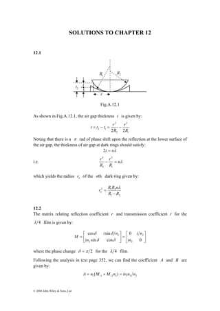
![sin 2 sin 2 8 3 × × =
δ θ 400 sin 4 sin
I = a = I +
max 0 I = 4I
θ =150o θ = 30o
© 2008 John Wiley & Sons, Ltd
21 22 3 2 B = (M +M n ) = in
A perfect anti-reflector requires:
0
in n n −
in
1 3 2 2 =
+
1 3 2 2
=
R A −
B
+
=
in n n in
A B
which gives:
2
2 n = n n
1 3
12.3
As shown in page 357 of the text, the intensity distribution of the interference pattern
is given by:
4 2 cos2 δ I = a
2
where δ is the phase difference between the two waves transmitted from the two
radio masts to a point P and is given by:
θ π θ
π
θ
π
λ
3 × 10 1500 ×
10
= kf = f =
so we have:
4 π 4 cos sin θ
0
2 2 π θ
2 [1 cos(4 sin )]
2
where 2
0 I = a represents the radiated intensity of each mast.
The intensity distribution is shown in the polar diagram below:
Fig.A.12.3
θ = 210o
θ = 0o
θ =180o
θ = 90o
θ = 270o
θ = 330o
I
θ](https://image.slidesharecdn.com/136253314-physics-of-vibration-and-waves-solutions-pain-141001200006-phpapp01/85/physics-of-vibration-and-waves-solutions-pain-144-320.jpg)
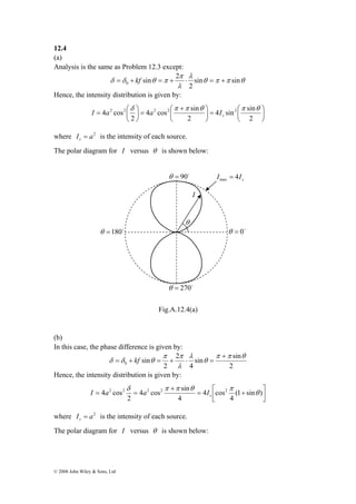
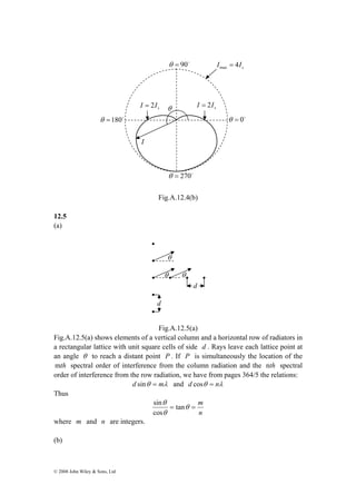
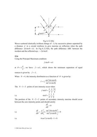
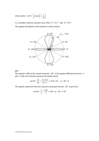
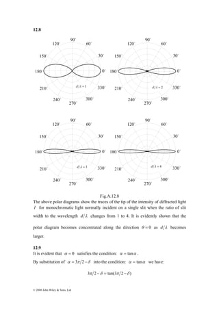
![Since N is a very large number, we have:
d d f f d f d
− −
dl −
© 2008 John Wiley & Sons, Ltd
d π
= ≈ 0
N
β
Then, suppose a non-monochromatic light, i.e. λ is not constant, incident on the
same grating, the phase change dβ required to move the diffracted light from the
principal maximum to the first minimum should be the same value as given above, so
we have:
sin π
(sin ) sin 1
π θ
= + ⎛ ⎟⎠
= ⎛
π θ
cos sin 0
π
2 = − = ≈
⎞
⎟⎠
⎜⎝
⎞
⎜⎝
N
f d f d
π
λ
λ
θ θ
λ
λ
θ π θ
λ
λ
β
which gives:
dθ = (nN cotθ )−1
12.12
(a)
The derivative of the equation:
f sinθ = nλ
gives:
f cosθdθ = ndλ
when θ is a small angle we have:
n
f
d θ
=
λ
d
When the diffracted light from the grating is projected by a lens of focal length F
on the screen, the relation between linear spacing on the screen l and the diffraction
angle θ is given by:
l = Fθ
Its derivative over λ gives:
nF
f
F d
dl θ
= =
d
d
λ
λ
(b)
Using the result given above, the change in linear separation per unit increase in
spectral order is given by:
7 7
2 (5.2 10 5 10 ) 2
2 10 [ ]
× × − ×
2 10
6
m
Fd
f
n
−
= ×
×
λ
= =](https://image.slidesharecdn.com/136253314-physics-of-vibration-and-waves-solutions-pain-141001200006-phpapp01/85/physics-of-vibration-and-waves-solutions-pain-151-320.jpg)
![12.13
(a)
Using the resolving power equation:
© 2008 John Wiley & Sons, Ltd
nN
λ
=
λ
d
we have:
328
7 7
− −
(5.89 × 10 + 5.896 ×
10 ) 2
λ
nd
= = − −
7 7
3 (5.896 10 5.89 10 )
≈
× × − ×
λ
N
(b)
Using the resolving power equation:
nN
λ
=
λ
d
we have:
7
6.5 ×
10 12
λ
d −
2.4 10 [ ]
3 9 10
4
m
nN
−
= ×
× ×
= =
λ
12.14
When the objects O and O′ are just resolved at I and I′ the principal
maximum of O and the first minimum of O′ are located at I . Rayleigh’s criterion
thus defines the path difference:
O′BI −O′AI = O′B −O′A = 1.22λ (BI = AI)
Also OB = OA giving
(O′B −OB) + (OA−O′A) = 1.22λ
Fig.Q.12.14 shows OA parallel to O′A and OB parallel to O′B , so:
OA−O′A = O′C = OO′sin i = s sin i
and
O′B −OB = O′C′ = OO′sin i = s sin i
We therefore write:
1.22λ
≈ or
i
s
2sin
1.22λ
= if i = 45o
i
s
2sin
O′ C C′
ii
O
i
A
B](https://image.slidesharecdn.com/136253314-physics-of-vibration-and-waves-solutions-pain-141001200006-phpapp01/85/physics-of-vibration-and-waves-solutions-pain-152-320.jpg)
![So, the momentum of these photons is given by:
1
h
E p
1
1
© 2008 John Wiley & Sons, Ltd
p = mc
Therefore, these photons’ spatial uncertainty should satisfy:
Δx ≥ h
mc
which shows the short wavelength limit on length measurement, i.e. the Compton wavelength, is
given by:
λ = h
mc
By substitution of electron mass: m 9.1 10 31[kg] e
= × − into the above equation, we have the
Compton wavelength for an electron given by:
34
6.63 10 12
2.42 10 [ ]
×
31 8
9.1 10 3 10
m
h
e
m c
−
−
−
≈ ×
× × ×
λ = =
13.3
The energy of a simple harmonic oscillation at frequency ω should satisfy:
E p + Δ
2 2
2
m 2 x 2
p
2
1
2
1
2 2
2
m x
m
m
Δ
= + ω ≥ ω
The relation:
4
( )( )
2
2 2 h Δx Δp ≈ gives:
2
2
Δ 2
≈ h
4 x
p
Δ
, by substitution into the above equation,
we have:
1
1
⎛ Δ
ω ω ω
ω ν
m x
m x
m x
m x
m x
m
2
2
2
8
2
2
2 8
2
2 2
2
2
2 2
2
2
2 2
2
= =
⎞
⎟⎠
⎜⎝
Δ
+ Δ ≥
Δ
+ Δ =
Δ
≥
h
h h
1
i.e. the simple harmonic oscillation has a minimum energy of hν
2
.
13.4
When an electron passes through a slit of width Δx , the intensity distribution of diffraction
pattern is given by:
2
2
0
sin
α
π
I α = I , where α = Δxsin
θ
λ
The first minimum of the intensity pattern occurs when α =π ,
π
i.e. θ π
α = Δxsin =
λ
Noting that λ = h p , we have:](https://image.slidesharecdn.com/136253314-physics-of-vibration-and-waves-solutions-pain-141001200006-phpapp01/85/physics-of-vibration-and-waves-solutions-pain-154-320.jpg)
![h
h
© 2008 John Wiley & Sons, Ltd
θ π
π
α = Δxpsin =
h
i.e. ΔxΔp = h
where Δp = psinθ is the change of the electron’s momentum in the direction parallel to the
plane of the slit. This relation is in accordance with Heisenberg’s uncertainty principle.
13.5
The angular spread due to diffraction can be seen as the half angular width of the principal
maximum Δθ of the diffraction pattern. Use the same analysis as Problem 13.4, we have:
α = d sin ≈ dΔ =
θ π
π
λ
θ
π
λ
10
5
−
λ
Δ = = = ≈ ′ −
i.e. 0.1 5 44
10
4
o
d
θ
13.6
The energy of the electron after acceleration across a potential difference V is given by:
E = eV , so its momentum is given by: p m E m eV e e = 2 = 2 , therefore its de Broglie
wavelength is given by:
1.23 10 [ ]
6.63 10
34
−
×
2 9.1 10 1.6 10
2
9 1 2
31 19
V m
m eV V
p
e
− −
− −
= ×
× × × ×
λ = = =
13.7
From problem 13.6 we have:
4.1
9 9
− −
1.23 10 1.23 10
1 2 =
3 10
10
×
×
=
×
= −
λ
V
∴V = 16.81[V]
13.8
The energy per unit volume of electromagnetic wave is given by: 2
E = 1ε E , where 0 E is the
2 0 0
electric field amplitude. For photons of zero rest mass, the energy is given by: E = mc2 = pc ,
where p is the average momentum per unit volume associated with this electromagnetic wave.
So we have:
1 2
2 0 0
E = pc
ε](https://image.slidesharecdn.com/136253314-physics-of-vibration-and-waves-solutions-pain-141001200006-phpapp01/85/physics-of-vibration-and-waves-solutions-pain-155-320.jpg)
![= 1ε
i.e. p E2 c
2 -2
F ⋅ V ⋅
m = ⋅ ⋅
P ε E I
1 1
6 11
1 hν = 1
× × −34 × × 11 = × −22 = × −3
© 2008 John Wiley & Sons, Ltd
2 0 0
The dimension the above equation is given by:
-1 -1
A ⋅ s ⋅ kg ⋅ m ⋅
m
-1 3
2 -2
C ⋅ W ⋅
m
1 -
-2
C V m
1 -
-2
1 -
kg m s
m s s A
m s A
⋅ ⋅
m s
m s
⋅ ⋅ ⋅
=
⋅ ⋅
=
⋅
=
⋅
which is the dimension of momentum.
13.9
When the wave is normally incident on a perfect absorber, all the photons’ velocity changes from
c to 0, the radiation pressure should equal the energy density of the incident wave, i.e.:
2
P = cp − 0 = cp = 1ε E
2 0 0
When the wave is normally incident on a perfect reflector, all the photons’ velocity changes to the
opposite directing but keeps the same value, hence, the radiation pressure is given by:
2
0 0 P = cp − (−cp) = 2cp =ε E
13.10
Using the result of Problem 13.9, we have the radiation pressure from the sun incident upon the
perfectly absorbing surface of the earth given by:
1.5 10 [Pa] 10 [atm]
1.4 ×
10
3 10
1
3
1
3
2
3
8
3
2
0 0
= × − ≈ −
×
= × = × = ×
c
13.11
Using the result of Problem 13.3, we have the minimum energy, i.e. the zero point energy, of such
an oscillation given by:
6.63 10 6.43 10 2.13 10 [J] 1.33 10 [eV]
2
2
13.12
The probability of finding the mass in the box is given by the integral:
4 4
⎛
x
π π
x
0.96
∫ ∫
− −
2 2
2
320
⎛
2 2
12
4 64
1 1
2 2
8
( ) 1 1
2 4
4
2
2
x
2
2
= − + ≈
⎞
⎟ ⎟⎠
⎜ ⎜⎝
= − +
⎞
⎟ ⎟⎠
⎜ ⎜⎝
= −
∫
−
π π
π
ψ
dx
a
a
a
dx
a
a
x dx
a
a
a
a
a
a
The general expression of the wave function is given by: ψ = Ceikx + De−ikx , where A,B are
constants. Using boundary condition at x = a and x = −a , we have:](https://image.slidesharecdn.com/136253314-physics-of-vibration-and-waves-solutions-pain-141001200006-phpapp01/85/physics-of-vibration-and-waves-solutions-pain-156-320.jpg)
![xyz dV c b a
A x
∫∫∫ ∫ ∫ ∫
y
π π π
( ) sin sin sin
z
dy z
π π π
⋅ ⎛ ⎟⎠
dx y
⋅ ⎛ ⎟⎠
A x
a a a
∫ ∫ ∫
sin sin sin
dx y
A x
cos 2 1
2
1
= ⎛
= ⎛ −
m = × − , the number of free electrons per unit volume in Copper is given by:
⎛ ⋅
⎞
⎡
28 34 3
⎤
= −
E n h
3 18
F m
© 2008 John Wiley & Sons, Ltd
1
2 2 2
dy z
cos 2
2
1
⎞
cos 2 1
2
π π π
⋅ ⎛ − 2
⎟⎠
1
⋅ ⎛ − 2
⎟⎠
1
2
2
0 0 0
2
0
2
0
2
0
2
2
0 0 0
2
2
= ⋅ ⋅ ⋅ =
⎞
⎟⎠
⎜⎝
⎞
⎜⎝
⎞
⎜⎝
⎟⎠
⎜⎝
⎞
⎜⎝
⎞
⎜⎝
=
∫ ∫ ∫
A a b c
dz
c
b
a
dz
c
b
a
dxdydz
c
b
a
a b c
ψ
i.e. A = 8 abc
13.14
Text in page 426 shows number of electrons per unit volume in energy interval dE is given by:
dE
2 × 4π (2 3 )1 2 1 2
=
dn m E 3
h
and the total number of electrons given by:
3 1 2 3 2
3
N 16 π
(2 me )
EF 3
h
=
so we have the total energy of these electrons given by:
F
U Edn E dn
∫ ∫
m E
= =
∫
2 ×
4 π
(2 )
0 3
3 1 2 5 2
F
E
E
NE
m E
16 (2 )
h
dE
h
dE
dE
f
f
3
5
5
3
3 1 2 3 2
0
=
π
= =
13.15
Noting that Copper has one conduction electron per atom and one atom has a mass of
1.66 10 27 kg
0
8 10 [m ]
9 ×
10
0 ≈ ×
= = m −
64 1.66 10
64
28 -3
27
3
0
× ×
n ρ
Using the expression of number of electrons per unit volume in text of page 426, we have the
Fermi energy level of Copper given by:
1.08 10 [J] 7[eV]
8 × 10 × 3 × (6.63 ×
10 )
16 2 (9.1 10 )
16 2
2 3
31 3
2 3
3
3
0 ≈ × =
⎥ ⎥
⎦
⎢ ⎢
⎣
× × ×
=
⎟ ⎟
⎠
⎜ ⎜
⎝
−
−
π π e](https://image.slidesharecdn.com/136253314-physics-of-vibration-and-waves-solutions-pain-141001200006-phpapp01/85/physics-of-vibration-and-waves-solutions-pain-158-320.jpg)
![13.16
By substitution of values of x , V − E , and m into the expression e−2αx , we have:
For an electron:
[ ] ( )
− − − × × ⎥⎦ −
= = = − ≈ ⎤
2 α 2 2 ( ) h 2 2 9.1 10 1.6 10 6.63 10 2 π
2 10 2.05 0.1
α h π
© 2008 John Wiley & Sons, Ltd
31 19 34 10
⎢⎣ ⎡
− − − − × × × × ×
e x e me V E x e e
For a proton:
[ ] 2 2 1.67 10 − 2 2 ( ) 27 1.6 10 − 19 ( 2 6.63 10 − 34 2 ) × 2 × 10 ⎥⎦ −
10
− 87.4 10 − ⎤
38
⎢⎣ ⎡
− = − − = − × × × × × = ≈
e e e e x mp V E x
13.17
Text in page 432-434 shows the amplitude reflection and transmission coefficients for such a
particle are given by:
k −
k
= = and
1 2
k k
1 2
r B
A
+
k
1 2
k k
1 2
t C
A
+
= =
where,
k 2mE
1 = and
h
k m E V
2 ( )
h
2
−
=
If V is a very large negative value at x > 0 , we have the amplitude reflection coefficient given
by:
1
r mE m E V
2 − 2 ( −
)
lim = −
2 + 2 ( −
)
=
→−∞ mE m E V
V
and the amplitude transmission coefficient given by:
0
t mE
lim 2 2 =
2 + 2 ( −
)
=
→−∞ mE m E V
V
i.e. the amplitude of reflected wave tends to unity and that of transmitted wave to zero.
13.18
The potential energy of one dimensional simple harmonic oscillator of frequency ω is given by:
V = 1 mω x
2 2
2
By substitution into Schrödinger’s equation, we have:
0
ψ m E m x
dx
2 1 2 2
+ ⎡ − ω ψ
2
2 2
2
⎤
= ⎥⎦
⎢⎣
d
h
(13.18.1)
Try 2 2 2 ψ (x) = a π e−a x in dψ dx :](https://image.slidesharecdn.com/136253314-physics-of-vibration-and-waves-solutions-pain-141001200006-phpapp01/85/physics-of-vibration-and-waves-solutions-pain-159-320.jpg)
![V dx
ψ ψ
Δ = = −
© 2008 John Wiley & Sons, Ltd
2 2
2 2
E p
2 8 sin
34 2
−
(6.63 10 )
31 10 2 2
8 × 9.1 × 10 × (0.91 × 10 ) ×
sin 65
19
8.88 10 [J] 55.5[eV]
= × =
×
=
= =
−
− −
o
e e r
r
r m a
h
m
θ
The difference between the incident and scattered kinetic energies is given by:
55.5 54 × = <
100% 2.8% 3.9%
−
54
=
E −
E
r i
E
i
13.21
For ψ = sin ka :
Since ψ ,ψ *,V are all periodic functions with a period of a , we have:
∞
Σ
∫
∫
=
Σ
kxV mx
sin cos 2
nx a mx
1 cos(2 )
∫
Σ
∫
∫
Σ
∫
∫
∫
∞
=
∞
=
∞
=
⎤
⎥⎦
π π
1 cos(2 )
nx
π
cos 2 cos 2
1
m n x
π π
m n x
mx
⎡ −
⎢⎣
+
+
=
− ⋅
= −
−
−
= −
1
0
1
0
1
0
0
1
0
2
0
2
*
*
cos 2 ( ) cos 2 ( )
1
2
2
2
2
cos 2
2
sin
m
a
m
m
a
m
m
a
a
m
m
a
a
m
a
dx
a
a
V
a
dx
a
a
V
nx a dx
dx
a
V
kxdx
dx
a
dx
E
π π
π
ψ ψ
The above equation has non-zero term only when m = n , so we have:
V a
1
⎞
⎟⎠
⎛ +
0 = =
n n
a
nx
cos 4 1
n V
a
a
dx
a
E V
2
2 2
⎜⎝
Δ =
∫ π
For ψ = cos ka :](https://image.slidesharecdn.com/136253314-physics-of-vibration-and-waves-solutions-pain-141001200006-phpapp01/85/physics-of-vibration-and-waves-solutions-pain-162-320.jpg)
![SOLUTIONS TO CHAPTER 14
14.1
For 30o 0 θ < , we have:
m ⎛ dx = ∫ x − ∫
x = ⎟⎠
− © 2008 John Wiley & Sons, Ltd
⎛
T T 1 1 = T ⎟ ⎟⎠
0
sin 2
30
4
0 1.017
2
⎞
⎜ ⎜⎝
< +
o
T T
i.e. 1.7% 2%
0
0 = <
−
T
For 90o 0 θ = , we have:
⎛
T T 1 1 = T ⎟ ⎟⎠
0
sin 2
90
4
0 1.125
2
⎞
⎜ ⎜⎝
= +
o
T T
i.e. 12.5%
0
0 =
−
T
14.2
Multiplying the equation of motion by 2dx dt and integrating with respect to t
gives:
m dx
⎛ ⎞
A x f x dx
dt
∫ − = ⎟⎠
⎜⎝
0
2
2 ( )
where A is the constant of integration. The velocity
dx is zero at the maximum
dt
2 ( ) x A f x dx .
displacement 0 x = x , giving = ∫ 0
0
2
0 f x dx f x dx F x F x
i.e. 2 ( ) 2 ( ) 2 ( ) 2 ( ) 0 0 0
dt
⎞
⎜⎝
dx = −
i.e. 2 [ ( ) ( )]
0 F x F x
dt m
Upon integration of the above equation, we have:](https://image.slidesharecdn.com/136253314-physics-of-vibration-and-waves-solutions-pain-141001200006-phpapp01/85/physics-of-vibration-and-waves-solutions-pain-164-320.jpg)
![⎤
⎡
⎞
⎛
⎞
⎛
− = + Σ∞
( ) 0
⎡
− Σ∞
=
3 1 9 1 a s − + a s − − +L= F
3 1 9 1 9 1 a s − − a s − + a s − +L= F
V V dV
© 2008 John Wiley & Sons, Ltd
t m dx
2 F ( x ) −
F ( x
) 0 = ∫
If x = 0 at time t = 0 and 0 τ is the period of oscillation, then 0 x = x at 4 0 t =τ ,
so we have:
τ m dx
∫ −
= 0
0 2 0
( ) ( )
0
4 x
F x F x
14.3
By substitution of the solution into &x& :
&x& a n nφ b n nφ
Σ∞
= − −
=
⎤
⎥⎦
⎡
⎢⎣
1
2 2
3
sin
n n
3 9
cos
n 9
Since 3 1 s << s , we have s x s x 1 ( ) ≈ , so:
x s x a s n n b s n n F t
n
n n φ φ cosω
3
sin
3 9
cos
9
1
2
1
2
1 = ⎥⎦
⎢⎣
⎟ ⎟⎠
⎜ ⎜⎝
− + ⎟ ⎟⎠
⎜ ⎜⎝
=
&&
⎤
⎞
⎛
⎞
⎛
i.e. φ φ cosφ
3
sin
3 9
cos
9 0
1
2
1
2
1 a s n n b s n n F
n
n n = ⎥⎦
⎢⎣
⎟ ⎟⎠
⎜ ⎜⎝
− + ⎟ ⎟⎠
⎜ ⎜⎝
i.e.
The above equation is true only if = 0 n b and the even numbered cosine terms are
zero. By neglecting the zero terms, we have:
( 1) cosφ ( 9) cos3φ cosφ 3 1 9 1 0 a s − + a s − +L= F
3
i.e. ( 1) cosφ ( 9)(4cos φ 3cosφ ) cosφ 0
3
i.e. [ ( 1) 3 ( 9)]cosφ 4 ( 9) cos φ cosφ 0
As we can see, only 3 a and 9 a are the main coefficients in the solution, i.e. the
fundamental frequency term and its third harmonic term are the significant terms in
the solution.
14.4
Since 0 V = V at 0 r = r , by expanding V at 0 r , we have:
⎞
r r d V
= + ⎛ 2
L + − ⎟ ⎟⎠
⎛
+ − ⎟⎠
⎜ ⎜⎝
⎞
⎜⎝
2 0
2
0 0 ( ) ( )
0 0
r r
dr
dr
r r](https://image.slidesharecdn.com/136253314-physics-of-vibration-and-waves-solutions-pain-141001200006-phpapp01/85/physics-of-vibration-and-waves-solutions-pain-165-320.jpg)
![© 2008 John Wiley & Sons, Ltd
2
2 u = p − p
2 1
2
2
ρ ρ ρ
1
1 2
−
ρ
(15.3.4)
Using equation 15.3.1 and 15.3.3 and the relation
e c T 1
p V −
1
γ ρ
= =
to eliminate 1 u gives:
⎞
⎟ ⎟⎠
⎛
2
2
2 γ 1 ρ ρ
ρ ρ u p p
⎜ ⎜⎝
−
2 2
−
=
−
1
1
2
2
1
2 2
1
γ
ρ
(15.3.5)
Then, using equation 15.3.4 and 15.3.5 to eliminate 2 u , we have:
2 1 ( )
1
2 1 p p
2 1
p p
1 2 2 1
−
−
ρ ρ γ
−
=
+
ρ ρ
γ
i.e.
1
p p ρ ρ
ρ ρ γ
2 1 2 1 2 1
2 1 1
2 1
−
−
−
=
+
p p
γ
i.e. [(1 ρ ρ )(γ 1) 2γ ] (1 ρ ρ )(γ 1) 2γβ 2 1 2 1 2 1 + − − p p = + − −
i.e. [ ( 1) ( 1)] ( 1) ( 1) 2 1 β γ − − γ + p p = γ − −β γ +
which yields:
β −
α
−
βα
p
=
1 1
2
p
where α = (γ −1) (γ +1) and 2 1 β = ρ ρ .
15.4
Using the result of Problems 15.1 and 15.2, we have:
( 1)
M
2
2
+
γ
( 1) 2
u
1
2
2
1
u
1 2
2
M = ⎛
u
*2 1
*
− +
⎞
= = = ⎟⎠
⎜⎝
s
s
M
u
u u
c
γ
(15.4.1)
Using equation 15.3.1 and 15.3.2 to eliminate 1 ρ
gives:
u
1
2
p p = −
−
ρ
1 2 1
2
2 2
u
u](https://image.slidesharecdn.com/136253314-physics-of-vibration-and-waves-solutions-pain-141001200006-phpapp01/85/physics-of-vibration-and-waves-solutions-pain-171-320.jpg)
![u 6
uu ut x xxx
2 tanh 12 tanh 8 tanh 12 tanh
= − − +
0
∂
∂
( , ) 2 log[1 x ct ] 2 e x ct 8 e x ct
u x t = − α − − α − = α − α
−
u 6
uu ut x xxx
2 3 2
uc u u u
2 tanh 12 tanh 8 tanh 12 tanh
= + + −
α φ α φ α φ α φ
3 3
u u
= − +
© 2008 John Wiley & Sons, Ltd
2 3 2
=
+ +
αuc φ αu φ α u φ αu φ
15.10
At the peak of Figure 15.5(a), φ = 2α (x − ct) = 0 , and near the base of Figure 15.5(a),
φ = 2α (x − ct) >> 0, i.e. e−φ ≈ 0 . Hence, the solution of the KdV equation can be written as:
2 ( ) 2 2 ( )
2
2
2 ( )
2
2
x
e
x
∂
+ ≈
∂
Then, we have the derivatives,
16 3 2 ( x ct)
t u = α ce− α −
64 5 2 ( x ct)
xxx u = − α e− α −
Therefore, if c = 4α 2 ,
+ = 0 t xxx u u
3
α15.11
Using the substitution z = x − ct and the relation tanh′φ ≡ sech2φ and sech′φ ≡ –sechφtanhφ,
where φ =α ( z − z ) 0 , we have the derivatives:
ut = –4α3c sech2φ tanhφ = 2αuc tanhφ
ux = –4 sech2φ tanhφ = –2αu tanhφ
uxx = 4 α4
sech4φ + 4α2u tanh2φ = 4α2u tanh2φ + u2
uxx = –16α5 sech2φ tanhφ + 48α5 sech4φ tanhφ = –8α3u tanhφ – 12αu2 tanhφ
Then, using the relation c = 4α 2 , we have:
0
8 tanh 8 tanh
=
− +
α φ α φ
15.12
If v v u x 2 + = , then:](https://image.slidesharecdn.com/136253314-physics-of-vibration-and-waves-solutions-pain-141001200006-phpapp01/85/physics-of-vibration-and-waves-solutions-pain-175-320.jpg)
![ψxx + (λ – u(x))ψ
= α2A sechα(x – x0) – 2α2A sech3α (x – x0) + [–α2 sech2α (x – x0)]A sechα (x – x0)
= 0
15.15
Using transformation u →u* −λ and x → x* + 6λt , where u* and x* are the variables
before transformation, we have: u* = u +λ and x* = x − 6λt , hence:
A
v c ⎛
εa y c ε a y
1 1
ε π cosπ
1 1 1 0 0
= + c a x
© 2008 John Wiley & Sons, Ltd
( * ) *t t t u = u −λ = u
u = ( u * −λ ) x∗ = u
*
x x * x x * * * *
u = u x = u
xx x*x* x x*x* = ∗ *
= ∗ * * * * * *
xxx x x x x x x x u u x u
Using the above relations, equation + 6 + = 0 t x xxx u uu u is transformed to its original form:
* 6 * * * 0
* * * * + + = t x x x x u u u u
15.16
Fig.A.15.16
In Fig.A.15.16, A is the peak and B is the base point of the leading edge of the right going
wave: y = asinπx . The phase velocity of any point on the leading edge is given by:
⎞
⎟⎠
= ⎛ + ⎟⎠
⎜⎝
⎞
⎛
⎜⎝
∂
∂
⎞
+ = ⎟⎠
⎜⎝
∂
∂
x
x
2
2
1 2
0
y = asinπx
D B](https://image.slidesharecdn.com/136253314-physics-of-vibration-and-waves-solutions-pain-141001200006-phpapp01/85/physics-of-vibration-and-waves-solutions-pain-177-320.jpg)
![π
∴ = ⎛ = =
A v c π
x
and phase velocity at : 1 1
© 2008 John Wiley & Sons, Ltd
⎞
(cos x cos -1)
B v c a
2
0
2
phase velocity at : cos cos
= ⎛ −
0
0
⎞
= = ⎟⎠
⎜⎝
⎜⎝
⎟⎠
ε π π π
B
A
∴phase velocity of A related to B :
1 1
− = − ⎛ − ε π ⎞
ε π 0 0 2 0
v v c c a c a du A B = = ⎟⎠
⎜⎝
1
2
The phase distance dx between A and B =π 2
∴Time for A to reach the position vertically above B is :
1 [secs]
π
= =
1 2
1
dx
du 2 c ε a π c ε
a
0 0](https://image.slidesharecdn.com/136253314-physics-of-vibration-and-waves-solutions-pain-141001200006-phpapp01/85/physics-of-vibration-and-waves-solutions-pain-178-320.jpg)