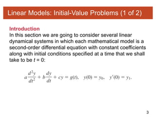
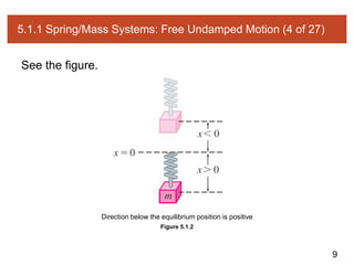
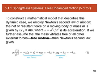
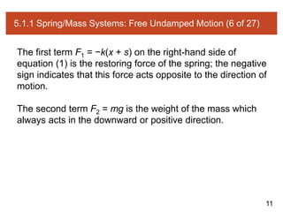
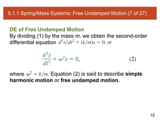
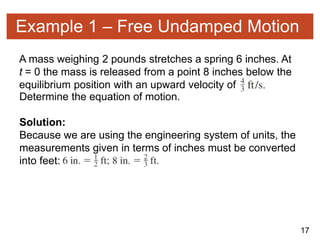
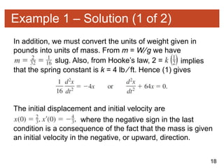
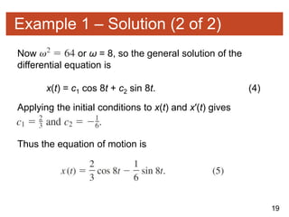
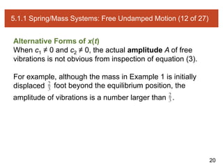
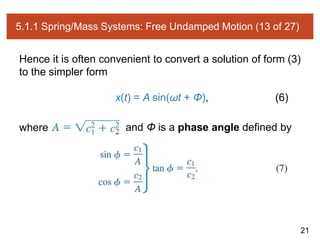
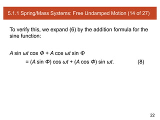
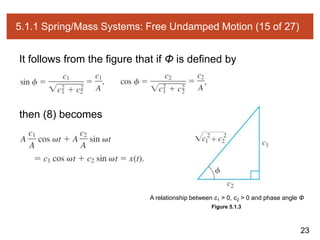
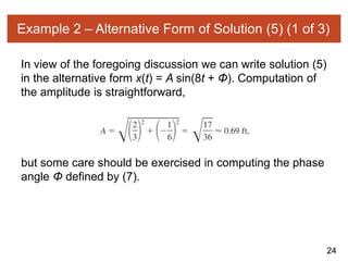
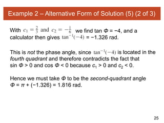
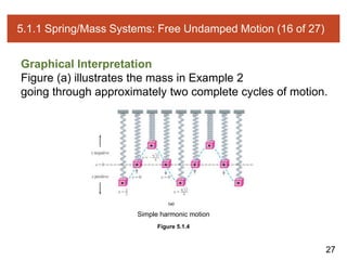
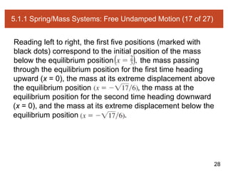
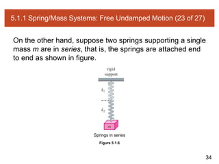
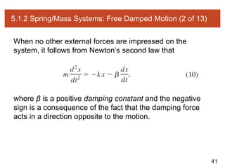
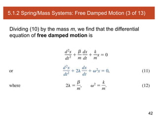
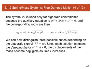
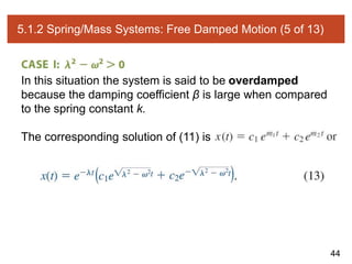
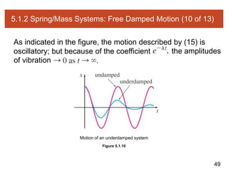
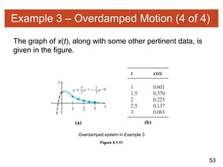
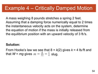
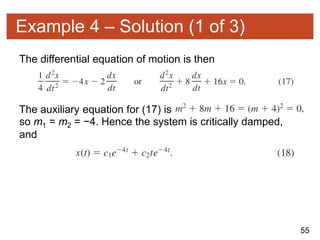
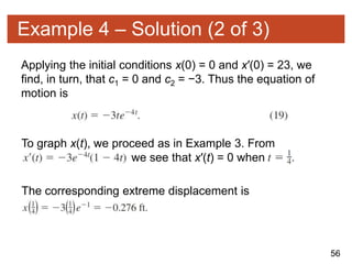
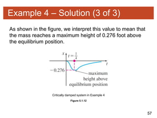
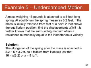
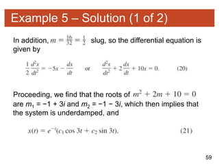
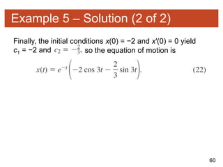
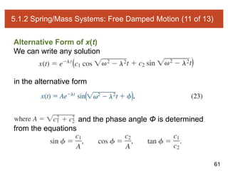
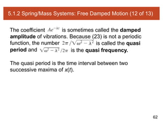
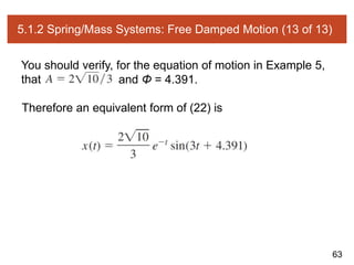
The document discusses modeling of electrical and mechanical systems. It provides examples of modeling an RLC network, DC motor, spring-mass-damper system, and closed-loop position control system using transfer functions derived from equations of motion. Transfer functions are obtained using Laplace transforms of differential equations describing the dynamics of the systems.
The document discusses modeling of electrical and mechanical systems. It provides examples of modeling translational and rotational mechanical systems including springs, masses, dampers, motors, and gears. It derives transfer functions for various systems using equations of motion and Laplace transforms. One example shows modeling a closed-loop position control system with a motor, gears, load, and position feedback.
APPLICATION OF HIGHER ORDER DIFFERENTIAL EQUATIONSAYESHA JAVED
1) The document discusses modeling and applications of second order differential equations. It provides examples of second order differential equations that model vibrating springs and electric current circuits.
2) Solving second order differential equations involves finding the complementary function and particular integral. The type of roots in the auxiliary equation determines the form of the complementary function.
3) An example solves a second order differential equation modeling a vibrating spring to find the position of a mass attached to the spring at any time.
This document summarizes a mechanical engineering student project analyzing the kinematics and dynamics of a forging manipulator. It includes:
1) Modeling the hydraulic actuators as spring-damper systems and computing kinematics using vector equations of the degrees of freedom.
2) Computing static preloads on the actuators to achieve equilibrium.
3) Linearizing the equations of motion around the equilibrium position to determine natural frequencies and mode shapes.
4) Calculating frequency response functions by solving the linearized equations with an external forcing function.
DOMV No 5 MATH MODELLING Newtonian d'Alembert Virtual Work (1).pdfahmedelsharkawy98
This document discusses different approaches for constructing mathematical models from physical systems:
1) Newtonian mechanics uses Newton's second law to directly obtain equations of motion for lumped mass systems.
2) D'Alembert's principle allows inertia forces to be included in equilibrium diagrams, making it useful for continuous systems.
3) The principle of virtual work equates the total virtual work done by internal and external forces during virtual displacements to zero, providing another approach for developing equations of motion. Examples are provided to illustrate Newtonian mechanics and the principle of virtual work.
This document discusses multi-degree-of-freedom (MDOF) systems and their analysis. It introduces concepts such as flexibility and stiffness matrices, natural frequencies and mode shapes, orthogonality of modes, and equations of motion. Methods for analyzing free and forced vibration of MDOF systems in the time domain are presented, including modal superposition and direct integration. An example 3DOF system is analyzed to illustrate the concepts.
The document introduces second order differential equations and their solutions. It defines an initial value problem for a second order equation as consisting of the equation and two initial conditions. Linear equations are introduced, which can be written in standard form or with constant or variable coefficients. The dynamical system formulation converts a second order equation to a system of first order equations. Undamped and damped free vibrations are discussed. Examples are provided, including finding the solution to an initial value problem, and determining the quasi-frequency, quasi-period, and equilibrium crossing time.
This chapter discusses vibration dynamics and methods for deriving equations of motion. The Newton-Euler and Lagrange methods are commonly used to derive equations of motion for vibrating systems. The Newton-Euler method is well-suited for discrete, lumped parameter models with a low degree of freedom. It involves drawing free body diagrams and applying Newton's second law to each mass to obtain the equations of motion. Having symmetric coefficient matrices is the main advantage of using the Lagrange method for mechanical vibrations.
This document discusses Lagrangian dynamics and Hamilton's principle. It begins by introducing important notation conventions used in the chapter. It then provides an overview of Hamilton's principle and how it can be used to derive Lagrange's equations of motion. This allows problems to be solved in a general manner even when forces are difficult to express or some constraints exist. Examples are provided, including deriving the equation of motion for a simple pendulum using both Cartesian and cylindrical coordinates. The concept of generalized coordinates is also introduced to represent the degrees of freedom of a system.
Lecture1 NPTEL for Basics of Vibrations for Simple Mechanical SystemsNaushad Ahamed
This document provides an introduction to vibrations and oscillations in mechanical systems. It discusses linear systems and how they relate an input signal to an output signal. As an example, it describes how forces acting on a vehicle excite vibrations that produce sound pressures in the passenger compartment. It then focuses on modeling single degree of freedom spring-mass and spring-mass-damper systems, providing the equations of motion for each and discussing how to determine the system parameters like stiffness from experiments. The key goals are to understand vibrations in simple mechanical systems using linear differential equations.
This document summarizes classical dynamics and small amplitude oscillations. It discusses oscillatory motion near equilibrium positions and developing the theory using Lagrange's equations. Normal modes of coupled oscillating systems are explored, where the normal coordinates represent eigenvectors that oscillate at characteristic frequencies. The principles of superposition and matrix representations are used to analyze examples like two coupled pendulums and a system of two masses connected by three springs.
1) A mass attached to a spring can move up and down from its equilibrium position. Its movement is modeled by a differential equation that depends on factors like the mass, spring constant, damping, and any external forcing.
2) There are three types of behavior for damped systems without external forcing: underdamped systems oscillate with a decaying amplitude, critically damped systems do not oscillate and cross the equilibrium at most once, and overdamped systems do not oscillate and may or may not cross the equilibrium.
3) For an undamped system with external periodic forcing, the behavior depends on whether the forcing frequency matches the natural frequency. If they are different, the displacement takes the form of a
I am Katherine Walters. I love exploring new topics. Academic writing seemed an exciting option for me. After working for many years with matlabassignmentexperts.com, I have assisted many students with their assignments. I can proudly say, each student I have served is happy with the quality of the solution that I have provided. I acquired my master's from the University of Sydney.
- A mass m is attached to one end of a horizontal spring, while the other end is anchored to a wall. The extension x(t) of the spring from its unstretched length determines the horizontal displacement of the mass.
- When undisturbed, the mass is at rest and the spring is unextended. But if displaced from this equilibrium, the spring exerts a restoring force f(x) = -kx on the mass according to Hooke's law, where k is the spring constant.
- Using Newton's second law, F=ma, this results in the mass undergoing simple harmonic motion described by the equation x(t) = A cos(ωt + Φ), where the frequency
This document provides background on analyzing the response of linear systems using modern tools from linear algebra. It introduces a simple spring-mass-damper system as an example and derives the equations of motion. The response depends on the damping ratio ζ. For ζ > 1, the system is overdamped with decaying exponential solutions. For ζ = 1, it is critically damped with a decaying exponential and linear term. For ζ < 1, it is underdamped with decaying sinusoidal oscillations. The document expresses the second-order system as a set of first-order equations and relates the free response to the eigenvalues and eigenvectors of the system matrix A. It then applies this framework to derive the
International Refereed Journal of Engineering and Science (IRJES)irjes
International Refereed Journal of Engineering and Science (IRJES) is a leading international journal for publication of new ideas, the state of the art research results and fundamental advances in all aspects of Engineering and Science. IRJES is a open access, peer reviewed international journal with a primary objective to provide the academic community and industry for the submission of half of original research and applications
1) This document provides two solutions to finding the acceleration of masses in an infinite Atwood's machine system.
2) The first solution shows that the acceleration of each subsequent mass is half the acceleration of the mass above it, with the top mass experiencing an acceleration of g/2.
3) The second solution models the system as an iterative function that approaches a fixed point of 3m, equivalent to two masses of m and 3m over the top pulley, also yielding a top acceleration of g/2.
Richard Feynman's high school physics teacher introduced him to the principle of least action, one of the most profound concepts in physics. The principle states that among all possible paths a physical system can take between two configurations, the actual path taken will be the one that minimizes the action. The action is defined as the time integral of the Lagrangian over the path, where the Lagrangian is the difference between the system's kinetic and potential energies. This principle allows physics to be formulated in terms of variational calculus and is the foundation for classical mechanics, electromagnetism, general relativity, and other physical theories.
Newton™s Laws; Moment of a Vector; Gravitation; Finite Rotations; Trajectory of a Projectile with Air Resistance; The Simple Pendulum; The Linear Harmonic Oscillator; The Damped Harmonic Oscillator
REPORT SUMMARYVibration refers to a mechanical.docxdebishakespeare
REPORT SUMMARY
Vibration refers to a mechanical phenomenon involving oscillations about a point. These oscillations can be of any imaginable range of amplitudes and frequencies, with each combination having its own effect. These effects can be positive and purposefully induced, but they can also be unintentional and catastrophic. It's therefore imperative to understand how to classify and model vibration.
Within the classroom portion of ME 345, we discussed damped and undamped vibrations, appropriate models, and several of their properties. The purpose of Lab 3 is to give us the corresponding "hands-on" experience to cement our understanding of the theory.
As it turns out, vibration can be modeled with a simple spring-mass system (spring-mass-damper system for damped vibration). In order to create a mathematical model for our simple spring-mass system, we apply Newton's second law and sum the forces about the mass. After applying some of our knowledge of differential equations, the result is a second order linear differential equation (in vector form). This can easily be converted to the scalar version, from which it's easy to glean various properties of the vibration (i.e. natural frequency, period, etc.).
In the lab, we were provided with a PASCO motion sensor, USB link, ramp, and accompanying software. All of the aforementioned equipment was already assembled and connected. The ramp was set up at an angle with a stop on the elevated end and the motion sensor on the lower end. The sensor was connected to the USB link, which was in turn connected to the computer. We chose to use the Xplorer GLX software to interface with the sensor and record our data. After receiving our equipment, we gathered data on our spring's extension with a known load to derive a spring constant. We were provided with a small cart to which we attached weights to increase its mass. In order to model free vibration, we placed the cart on the track and attached it to the stop at the top of the ramp with a spring. After displacing the cart a certain distance from its equilibrium point, the cart was released and was allowed to oscillate on the track while we recorded its distance from the sensor. This was done with displacements of -20cm, -10cm, +10cm, and +20cm from the system's equilibrium point. After gathering this data for the "free" case, a magnet was attached to the front of the car, spaced as far from the track as possible. As the track is magnetic, this caused a slight damping effect, basically converting our spring-mass system to an underdamped spring-mass-damper system. After repeating the procedure for the "free" case, we moved the magnets as close to the track as possible (causing the system to become overdamped) and again repeated the procedure for the "free" case.
We were finally able to determine the period, phase angle, damping coefficients, and circular and cyclical frequencies for the three systems. There were similarities and differ ...
The document outlines the plan for a lecture on state-space models of systems and linearization. It will begin with a review of control and feedback concepts. The main topic will be introducing state-space models, which provide a general framework for representing different types of systems with differential equations. Examples will be used to illustrate how to derive state-space models from physical systems like masses on springs, electrical circuits, and pendulums. The goal is for students to master the state-space modeling approach in order to enable later analysis and design of systems.
On the Application of the Fixed Point Theory to the Solution of Systems of Li...BRNSS Publication Hub
This document discusses solving systems of linear differential equations and their applications to biological and physical problems. It begins by introducing systems of linear differential equations and rewriting them in matrix form. It then covers some key results from the theory of first-order linear systems, including how any nth-order linear differential equation can be converted to an equivalent first-order system. It also discusses properties of the solution space for homogeneous systems and methods for solving non-homogeneous systems. The document aims to illustrate the underlying theories of linear systems of differential equations through examples and applications to problems in cell biology and physics.
This document discusses solving systems of linear differential equations and their applications to biological and physical problems. It begins by defining systems of linear differential equations and rewriting them in matrix form. It then covers results from the general theory of first-order systems, including theorems on existence and uniqueness of solutions. It also discusses transforming nth-order equations into first-order systems and properties of the solution space. Applications to cell biology and physics are mentioned.
This document discusses solving systems of linear differential equations and their applications to biological and physical problems. It begins by defining systems of linear differential equations and rewriting them in matrix form. It then covers results from the general theory of first-order systems, including theorems on existence and uniqueness of solutions. It also discusses transforming nth-order differential equations into equivalent first-order systems and properties of the solution space. The document concludes by briefly mentioning methods for solving non-homogeneous first-order systems.
The document discusses oscillations and simple harmonic motion. It defines periodic motion, oscillatory motion, and harmonic motion. Harmonic motion can be described using sine and cosine functions. Examples of oscillations include a swinging pendulum and vibrating springs. The period and frequency of oscillations are defined. For simple harmonic motion, the displacement is directly proportional to the displacement from equilibrium and opposite in sign. The velocity and acceleration functions for SHM are derived. For a mass-spring system, the restoring force is proportional to the displacement. The total mechanical energy of a simple harmonic oscillator remains constant over time as the kinetic and potential energy alternately increase and decrease during oscillation.
Similar to ModelingZillDiffEQ9_LecturePPTs_05_01.pptx (20)
An improved modulation technique suitable for a three level flying capacitor ...IJECEIAES
This research paper introduces an innovative modulation technique for controlling a 3-level flying capacitor multilevel inverter (FCMLI), aiming to streamline the modulation process in contrast to conventional methods. The proposed
simplified modulation technique paves the way for more straightforward and
efficient control of multilevel inverters, enabling their widespread adoption and
integration into modern power electronic systems. Through the amalgamation of
sinusoidal pulse width modulation (SPWM) with a high-frequency square wave
pulse, this controlling technique attains energy equilibrium across the coupling
capacitor. The modulation scheme incorporates a simplified switching pattern
and a decreased count of voltage references, thereby simplifying the control
algorithm.
Introduction- e - waste – definition - sources of e-waste– hazardous substances in e-waste - effects of e-waste on environment and human health- need for e-waste management– e-waste handling rules - waste minimization techniques for managing e-waste – recycling of e-waste - disposal treatment methods of e- waste – mechanism of extraction of precious metal from leaching solution-global Scenario of E-waste – E-waste in India- case studies.
Redefining brain tumor segmentation: a cutting-edge convolutional neural netw...IJECEIAES
Medical image analysis has witnessed significant advancements with deep learning techniques. In the domain of brain tumor segmentation, the ability to
precisely delineate tumor boundaries from magnetic resonance imaging (MRI)
scans holds profound implications for diagnosis. This study presents an ensemble convolutional neural network (CNN) with transfer learning, integrating
the state-of-the-art Deeplabv3+ architecture with the ResNet18 backbone. The
model is rigorously trained and evaluated, exhibiting remarkable performance
metrics, including an impressive global accuracy of 99.286%, a high-class accuracy of 82.191%, a mean intersection over union (IoU) of 79.900%, a weighted
IoU of 98.620%, and a Boundary F1 (BF) score of 83.303%. Notably, a detailed comparative analysis with existing methods showcases the superiority of
our proposed model. These findings underscore the model’s competence in precise brain tumor localization, underscoring its potential to revolutionize medical
image analysis and enhance healthcare outcomes. This research paves the way
for future exploration and optimization of advanced CNN models in medical
imaging, emphasizing addressing false positives and resource efficiency.
Applications of artificial Intelligence in Mechanical Engineering.pdfAtif Razi
Historically, mechanical engineering has relied heavily on human expertise and empirical methods to solve complex problems. With the introduction of computer-aided design (CAD) and finite element analysis (FEA), the field took its first steps towards digitization. These tools allowed engineers to simulate and analyze mechanical systems with greater accuracy and efficiency. However, the sheer volume of data generated by modern engineering systems and the increasing complexity of these systems have necessitated more advanced analytical tools, paving the way for AI.
AI offers the capability to process vast amounts of data, identify patterns, and make predictions with a level of speed and accuracy unattainable by traditional methods. This has profound implications for mechanical engineering, enabling more efficient design processes, predictive maintenance strategies, and optimized manufacturing operations. AI-driven tools can learn from historical data, adapt to new information, and continuously improve their performance, making them invaluable in tackling the multifaceted challenges of modern mechanical engineering.
Null Bangalore | Pentesters Approach to AWS IAMDivyanshu
#Abstract:
- Learn more about the real-world methods for auditing AWS IAM (Identity and Access Management) as a pentester. So let us proceed with a brief discussion of IAM as well as some typical misconfigurations and their potential exploits in order to reinforce the understanding of IAM security best practices.
- Gain actionable insights into AWS IAM policies and roles, using hands on approach.
#Prerequisites:
- Basic understanding of AWS services and architecture
- Familiarity with cloud security concepts
- Experience using the AWS Management Console or AWS CLI.
- For hands on lab create account on [killercoda.com](https://killercoda.com/cloudsecurity-scenario/)
# Scenario Covered:
- Basics of IAM in AWS
- Implementing IAM Policies with Least Privilege to Manage S3 Bucket
- Objective: Create an S3 bucket with least privilege IAM policy and validate access.
- Steps:
- Create S3 bucket.
- Attach least privilege policy to IAM user.
- Validate access.
- Exploiting IAM PassRole Misconfiguration
-Allows a user to pass a specific IAM role to an AWS service (ec2), typically used for service access delegation. Then exploit PassRole Misconfiguration granting unauthorized access to sensitive resources.
- Objective: Demonstrate how a PassRole misconfiguration can grant unauthorized access.
- Steps:
- Allow user to pass IAM role to EC2.
- Exploit misconfiguration for unauthorized access.
- Access sensitive resources.
- Exploiting IAM AssumeRole Misconfiguration with Overly Permissive Role
- An overly permissive IAM role configuration can lead to privilege escalation by creating a role with administrative privileges and allow a user to assume this role.
- Objective: Show how overly permissive IAM roles can lead to privilege escalation.
- Steps:
- Create role with administrative privileges.
- Allow user to assume the role.
- Perform administrative actions.
- Differentiation between PassRole vs AssumeRole
Try at [killercoda.com](https://killercoda.com/cloudsecurity-scenario/)
Comparative analysis between traditional aquaponics and reconstructed aquapon...bijceesjournal
The aquaponic system of planting is a method that does not require soil usage. It is a method that only needs water, fish, lava rocks (a substitute for soil), and plants. Aquaponic systems are sustainable and environmentally friendly. Its use not only helps to plant in small spaces but also helps reduce artificial chemical use and minimizes excess water use, as aquaponics consumes 90% less water than soil-based gardening. The study applied a descriptive and experimental design to assess and compare conventional and reconstructed aquaponic methods for reproducing tomatoes. The researchers created an observation checklist to determine the significant factors of the study. The study aims to determine the significant difference between traditional aquaponics and reconstructed aquaponics systems propagating tomatoes in terms of height, weight, girth, and number of fruits. The reconstructed aquaponics system’s higher growth yield results in a much more nourished crop than the traditional aquaponics system. It is superior in its number of fruits, height, weight, and girth measurement. Moreover, the reconstructed aquaponics system is proven to eliminate all the hindrances present in the traditional aquaponics system, which are overcrowding of fish, algae growth, pest problems, contaminated water, and dead fish.
Electric vehicle and photovoltaic advanced roles in enhancing the financial p...IJECEIAES
Climate change's impact on the planet forced the United Nations and governments to promote green energies and electric transportation. The deployments of photovoltaic (PV) and electric vehicle (EV) systems gained stronger momentum due to their numerous advantages over fossil fuel types. The advantages go beyond sustainability to reach financial support and stability. The work in this paper introduces the hybrid system between PV and EV to support industrial and commercial plants. This paper covers the theoretical framework of the proposed hybrid system including the required equation to complete the cost analysis when PV and EV are present. In addition, the proposed design diagram which sets the priorities and requirements of the system is presented. The proposed approach allows setup to advance their power stability, especially during power outages. The presented information supports researchers and plant owners to complete the necessary analysis while promoting the deployment of clean energy. The result of a case study that represents a dairy milk farmer supports the theoretical works and highlights its advanced benefits to existing plants. The short return on investment of the proposed approach supports the paper's novelty approach for the sustainable electrical system. In addition, the proposed system allows for an isolated power setup without the need for a transmission line which enhances the safety of the electrical network
3. 3
Linear Models: Initial-Value Problems (1 of 2)
Introduction
In this section we are going to consider several linear
dynamical systems in which each mathematical model is a
second-order differential equation with constant coefficients
along with initial conditions specified at a time that we shall
take to be t = 0:
4. 4
Linear Models: Initial-Value Problems (2 of 2)
The function g is variously called the driving function,
forcing function, or input of the system.
A solution y(t) of the differential equation on an interval I
containing t = 0 that satisfies the initial conditions is called
the response or output of the system.
6. 6
5.1.1 Spring/Mass Systems: Free Undamped Motion (1 of 27)
Newton’s Second Law
When a mass m is attached to the lower end of a spring of
negligible mass, it stretches the spring by an amount s and
attains an equilibrium position (or rest position) at which its
weight W is balanced by the restoring force ks of the spring.
7. 7
5.1.1 Spring/Mass Systems: Free Undamped Motion (2 of 27)
As indicated in the figure the condition of equilibrium is
mg = ks or mg − ks = 0.
Figure 5.1.1
Spring/mass system
8. 8
5.1.1 Spring/Mass Systems: Free Undamped Motion (3 of 27)
Now suppose the mass on the spring is set in motion by
giving it an initial displacement (an elongation or a
compression) and an initial velocity.
Let us assume that the motion takes place in a vertical line,
that the displacements x(t) of the mass are measured along
this line such that x = 0 corresponds to the equilibrium
position, and that displacements measured below the
equilibrium position are positive.
9. 9
5.1.1 Spring/Mass Systems: Free Undamped Motion (4 of 27)
See the figure.
Figure 5.1.2
Direction below the equilibrium position is positive
10. 10
5.1.1 Spring/Mass Systems: Free Undamped Motion (5 of 27)
To construct a mathematical model that describes this
dynamic case, we employ Newton’s second law of motion:
the net or resultant force on a moving body of mass m is
given by ΣFk = ma, where is its acceleration. If we
further assume that the mass vibrates free of all other
external forces—free motion—then Newton’s second law
gives
11. 11
5.1.1 Spring/Mass Systems: Free Undamped Motion (6 of 27)
The first term F1 = −k(x + s) on the right-hand side of
equation (1) is the restoring force of the spring; the negative
sign indicates that this force acts opposite to the direction of
motion.
The second term F2 = mg is the weight of the mass which
always acts in the downward or positive direction.
12. 12
5.1.1 Spring/Mass Systems: Free Undamped Motion (7 of 27)
DE of Free Undamped Motion
By dividing (1) by the mass m, we obtain the second-order
differential equation
where Equation (2) is said to describe simple
harmonic motion or free undamped motion.
13. 13
5.1.1 Spring/Mass Systems: Free Undamped Motion (8 of 27)
Two obvious initial conditions associated with (2) are
x(0) = x0 and x′(0) = x1, the initial displacement and initial
velocity of the mass, respectively.
Equation of Motion
To solve equation (2), we note that the solutions of its
auxiliary equation are the complex numbers
m1 = ωi, m2 = −ωi.
14. 14
5.1.1 Spring/Mass Systems: Free Undamped Motion (9 of 27)
Thus from
we find the general solution of (2) to be
x(t) = c1 cos ωt + c2 sin ωt. (3)
The period of motion described by (3) is T = 2π∕ω. The
number T represents the time (measured in seconds) it
takes the mass to execute one cycle of motion.
15. 15
5.1.1 Spring/Mass Systems: Free Undamped Motion (10 of 27)
The frequency of motion is f = 1 ∕ T = ω∕2π and is the
number of cycles completed each second. For example, if
x(t) = 2 cos 3πt − 4 sin 3πt, then the period is
T = 2π∕3π = 2 ∕ 3 s, and the frequency is f = 3 ∕ 2 cycles/s.
From a graphical viewpoint the graph of x(t) repeats every
second, that is, cycles of the graph
are completed each second (or, equivalently, three cycles of
the graph are completed every 2 seconds).
16. 16
5.1.1 Spring/Mass Systems: Free Undamped Motion (11 of 27)
The number (measured in radians per second)
is called the circular frequency of the system.
Finally, when the initial conditions are used to determine the
constants c1 and c2 in (3), we say that the resulting
particular solution or response is the equation of motion.
17. 17
Example 1 – Free Undamped Motion
A mass weighing 2 pounds stretches a spring 6 inches. At
t = 0 the mass is released from a point 8 inches below the
equilibrium position with an upward velocity of
Determine the equation of motion.
Solution:
Because we are using the engineering system of units, the
measurements given in terms of inches must be converted
into feet:
18. 18
Example 1 – Solution (1 of 2)
In addition, we must convert the units of weight given in
pounds into units of mass. From m = W∕g we have
slug. Also, from Hooke’s law, 2 = implies
that the spring constant is k = 4 lb ∕ ft. Hence (1) gives
The initial displacement and initial velocity are
where the negative sign in the last
condition is a consequence of the fact that the mass is given
an initial velocity in the negative, or upward, direction.
19. 19
Example 1 – Solution (2 of 2)
Now or ω = 8, so the general solution of the
differential equation is
x(t) = c1 cos 8t + c2 sin 8t. (4)
Applying the initial conditions to x(t) and x′(t) gives
Thus the equation of motion is
20. 20
5.1.1 Spring/Mass Systems: Free Undamped Motion (12 of 27)
Alternative Forms of x(t)
When c1 ≠ 0 and c2 ≠ 0, the actual amplitude A of free
vibrations is not obvious from inspection of equation (3).
For example, although the mass in Example 1 is initially
displaced foot beyond the equilibrium position, the
amplitude of vibrations is a number larger than .
21. 21
5.1.1 Spring/Mass Systems: Free Undamped Motion (13 of 27)
Hence it is often convenient to convert a solution of form (3)
to the simpler form
x(t) = A sin(ωt + Φ), (6)
where and Φ is a phase angle defined by
22. 22
5.1.1 Spring/Mass Systems: Free Undamped Motion (14 of 27)
To verify this, we expand (6) by the addition formula for the
sine function:
A sin ωt cos Φ + A cos ωt sin Φ
= (A sin Φ) cos ωt + (A cos Φ) sin ωt. (8)
23. 23
5.1.1 Spring/Mass Systems: Free Undamped Motion (15 of 27)
It follows from the figure that if Φ is defined by
then (8) becomes
Figure 5.1.3
A relationship between c1 > 0, c2 > 0 and phase angle Φ
24. 24
Example 2 – Alternative Form of Solution (5) (1 of 3)
In view of the foregoing discussion we can write solution (5)
in the alternative form x(t) = A sin(8t + Φ). Computation of
the amplitude is straightforward,
but some care should be exercised in computing the phase
angle Φ defined by (7).
25. 25
Example 2 – Alternative Form of Solution (5) (2 of 3)
With we find tan Φ = −4, and a
calculator then gives = −1.326 rad.
This is not the phase angle, since is located in the
fourth quadrant and therefore contradicts the fact that
sin Φ > 0 and cos Φ < 0 because c1 > 0 and c2 < 0.
Hence we must take Φ to be the second-quadrant angle
Φ = π + (−1.326) = 1.816 rad.
26. 26
Example 2 – Alternative Form of Solution (5) (3 of 3)
Thus (5) is the same as
The period of this function is T = 2π ∕ 8 = π∕4 s.
27. 27
5.1.1 Spring/Mass Systems: Free Undamped Motion (16 of 27)
Graphical Interpretation
Figure (a) illustrates the mass in Example 2
going through approximately two complete cycles of motion.
Figure 5.1.4
Simple harmonic motion
28. 28
5.1.1 Spring/Mass Systems: Free Undamped Motion (17 of 27)
Reading left to right, the first five positions (marked with
black dots) correspond to the initial position of the mass
below the equilibrium position the mass passing
through the equilibrium position for the first time heading
upward (x = 0), the mass at its extreme displacement above
the equilibrium position , the mass at the
equilibrium position for the second time heading downward
(x = 0), and the mass at its extreme displacement below the
equilibrium position .
29. 29
5.1.1 Spring/Mass Systems: Free Undamped Motion (18 of 27)
The black dots on the graph of (9), given in figure (b), also
agree with the five positions just given.
Figure 5.1.4
Simple harmonic motion
30. 30
5.1.1 Spring/Mass Systems: Free Undamped Motion (19 of 27)
Note, however, that in Figure 5.1.4(b) the positive direction in
the tx-plane is the usual upward direction and so is opposite
to the positive direction indicated in Figure 5.1.4(a).
Hence the solid blue graph representing the motion of the
mass in Figure 5.1.4(b) is the reflection through the t-axis of
the blue dashed curve in Figure 5.1.4(a).
31. 31
5.1.1 Spring/Mass Systems: Free Undamped Motion (20 of 27)
Form (6) is very useful because it is easy to find values of
time for which the graph of x(t) crosses the positive t-axis
(the line x = 0).
We observe that sin(ωt + Φ) = 0 when ωt + Φ = nπ, where n
is a nonnegative integer.
32. 32
5.1.1 Spring/Mass Systems: Free Undamped Motion (21 of 27)
Double Spring Systems
Suppose two parallel springs, with constants k1 and k2, are
attached to a common rigid support and then to a single
mass m as shown in figure.
Figure 5.1.5
Parallel springs
33. 33
5.1.1 Spring/Mass Systems: Free Undamped Motion (22 of 27)
If the mass is displaced from its equilibrium position, the
displacement x is the same for both springs and so the net
restoring force of the spring in (1) is simply
−k1x − k2x = −(k1 + k2)x.
We say that
keff = k1 + k2
is the effective spring constant of the system.
34. 34
5.1.1 Spring/Mass Systems: Free Undamped Motion (23 of 27)
On the other hand, suppose two springs supporting a single
mass m are in series, that is, the springs are attached end
to end as shown in figure.
Figure 5.1.6
Springs in series
35. 35
5.1.1 Spring/Mass Systems: Free Undamped Motion (24 of 27)
In this case, a displacement x of the mass from its
equilibrium consists of the sum x = x1 + x2, where x1 and x2
are the displacements of the respective springs.
But the restoring force is the same for both springs, so if keff
is the effective spring constant of the system we have
−keff(x1 + x2) = −k1x1 = −k2x2.
36. 36
5.1.1 Spring/Mass Systems: Free Undamped Motion (25 of 27)
From k1x1 = k2x2 we see x1 = (k2 ∕k1)x2 and so
−keff (x1 + x2) = −k2x2 is the same as
Solving the last equation for keff yields
So in either of the above cases, the differential equation of
motion is (1) with k replaced by keff.
37. 37
5.1.1 Spring/Mass Systems: Free Undamped Motion (26 of 27)
Systems with Variable Spring Constants
In the model discussed above we assumed an ideal world—
a world in which the physical characteristics of the spring do
not change over time.
In the nonideal world, however, it seems reasonable to
expect that when a spring/mass system is in motion for a
long period, the spring will weaken; in other words, the
“spring constant” will vary—or, more specifically, decay—
with time.
38. 38
5.1.1 Spring/Mass Systems: Free Undamped Motion (27 of 27)
In one model for the aging spring the spring constant k in
(1) is replaced by the decreasing function k > 0,
α > 0.
When a spring/mass system is subjected to an environment
in which the temperature is rapidly decreasing, it might
make sense to replace the constant k with K(t) = kt, k > 0, a
function that increases with time.
The resulting model, mx″ + ktx = 0, is a form of Airy’s
differential equation.
40. 40
5.1.2 Spring/Mass Systems: Free Damped Motion (1 of 13)
DE of Free Damped Motion
In the study of mechanics, damping forces acting on a body
are considered to be proportional to a power of the
instantaneous velocity.
In particular, we shall assume throughout the subsequent
discussion that this force is given by a constant multiple of
dx∕dt.
41. 41
5.1.2 Spring/Mass Systems: Free Damped Motion (2 of 13)
When no other external forces are impressed on the
system, it follows from Newton’s second law that
where β is a positive damping constant and the negative
sign is a consequence of the fact that the damping force
acts in a direction opposite to the motion.
42. 42
5.1.2 Spring/Mass Systems: Free Damped Motion (3 of 13)
Dividing (10) by the mass m, we find that the differential
equation of free damped motion is
43. 43
5.1.2 Spring/Mass Systems: Free Damped Motion (4 of 13)
The symbol 2λ is used only for algebraic convenience
because the auxiliary equation is and
the corresponding roots are then
We can now distinguish three possible cases depending on
the algebraic sign of Since each solution contains
the damping factor λ > 0, the displacements of the
mass become negligible as time t increases.
44. 44
5.1.2 Spring/Mass Systems: Free Damped Motion (5 of 13)
In this situation the system is said to be overdamped
because the damping coefficient β is large when compared
to the spring constant k.
The corresponding solution of (11) is
45. 45
5.1.2 Spring/Mass Systems: Free Damped Motion (6 of 13)
This equation represents a smooth and nonoscillatory
motion. The figure shows two possible graphs of x(t).
Figure 5.1.8
Motion of an overdamped system
46. 46
5.1.2 Spring/Mass Systems: Free Damped Motion (7 of 13)
The system is said to be critically damped because any
slight decrease in the damping force would result in
oscillatory motion.
The general solution of (11) is
47. 47
5.1.2 Spring/Mass Systems: Free Damped Motion (8 of 13)
Some graphs of typical motion are given in the figure.
Figure 5.1.9
Motion of a critically damped system
Notice that the motion is quite similar to that of an
overdamped system. It is also apparent from (14) that the
mass can pass through the equilibrium position at most one
time.
48. 48
5.1.2 Spring/Mass Systems: Free Damped Motion (9 of 13)
In this case the system is said to be underdamped, since
the damping coefficient is small in comparison to the spring
constant. The roots m1 and m2 are now complex:
Thus the general solution of equation (11) is
49. 49
5.1.2 Spring/Mass Systems: Free Damped Motion (10 of 13)
As indicated in the figure, the motion described by (15) is
oscillatory; but because of the coefficient the amplitudes
of vibration
Figure 5.1.10
Motion of an underdamped system
50. 50
Example 3 – Overdamped Motion (1 of 4)
It is readily verified that the solution of the initial-value
problem
The problem can be interpreted as representing the
overdamped motion of a mass on a spring. The mass is
initially released from a position 1 unit below the
equilibrium position with a downward velocity of 1 ft∕s.
51. 51
Example 3 – Overdamped Motion (2 of 4)
To graph x(t), we find the value of t for which the function
has an extremum—that is, the value of time for which the
first derivative (velocity) is zero. Differentiating (16) gives
so x′(t) = 0 implies that
It follows from the first derivative test, as well as our
physical intuition, that x(0.157) = 1.069 ft is actually a
maximum. In other words, the mass attains an extreme
displacement of 1.069 feet below the equilibrium position.
52. 52
Example 3 – Overdamped Motion (3 of 4)
We should also check to see whether the graph crosses the
t-axis—that is, whether the mass passes through the
equilibrium position. This cannot happen in this instance
because the equation x(t) = 0, or has the physically
irrelevant solution
53. 53
Example 3 – Overdamped Motion (4 of 4)
The graph of x(t), along with some other pertinent data, is
given in the figure.
Figure 5.1.11
Overdamped system in Example 3
54. 54
Example 4 – Critically Damped Motion
A mass weighing 8 pounds stretches a spring 2 feet.
Assuming that a damping force numerically equal to 2 times
the instantaneous velocity acts on the system, determine
the equation of motion if the mass is initially released from
the equilibrium position with an upward velocity of 3 ft∕s.
Solution:
From Hooke’s law we see that 8 = k(2) gives k = 4 lb∕ft and
that W = mg gives slug.
55. 55
Example 4 – Solution (1 of 3)
The differential equation of motion is then
The auxiliary equation for (17) is
so m1 = m2 = −4. Hence the system is critically damped,
and
56. 56
Example 4 – Solution (2 of 3)
Applying the initial conditions x(0) = 0 and x′(0) = 23, we
find, in turn, that c1 = 0 and c2 = −3. Thus the equation of
motion is
To graph x(t), we proceed as in Example 3. From
we see that x′(t) = 0 when
The corresponding extreme displacement is
57. 57
Example 4 – Solution (3 of 3)
As shown in the figure, we interpret this value to mean that
the mass reaches a maximum height of 0.276 foot above
the equilibrium position.
Figure 5.1.12
Critically damped system in Example 4
58. 58
Example 5 – Underdamped Motion
A mass weighing 16 pounds is attached to a 5-foot-long
spring. At equilibrium the spring measures 8.2 feet. If the
mass is initially released from rest at a point 2 feet above
the equilibrium position, find the displacements x(t) if it is
further known that the surrounding medium offers a
resistance numerically equal to the instantaneous velocity.
Solution:
The elongation of the spring after the mass is attached is
8.2 − 5 = 3.2 ft, so it follows from Hooke’s law that
16 = k(3.2) or k = 5 lb∕ft.
59. 59
Example 5 – Solution (1 of 2)
In addition, slug, so the differential equation is
given by
Proceeding, we find that the roots of
are m1 = −1 + 3i and m2 = −1 − 3i, which then implies that
the system is underdamped, and
60. 60
Example 5 – Solution (2 of 2)
Finally, the initial conditions x(0) = −2 and x′(0) = 0 yield
c1 = −2 and so the equation of motion is
61. 61
5.1.2 Spring/Mass Systems: Free Damped Motion (11 of 13)
Alternative Form of x(t)
We can write any solution
in the alternative form
and the phase angle Φ is determined
from the equations
62. 62
5.1.2 Spring/Mass Systems: Free Damped Motion (12 of 13)
The coefficient is sometimes called the damped
amplitude of vibrations. Because (23) is not a periodic
function, the number is called the quasi
period and is the quasi frequency.
The quasi period is the time interval between two
successive maxima of x(t).
63. 63
5.1.2 Spring/Mass Systems: Free Damped Motion (13 of 13)
You should verify, for the equation of motion in Example 5,
that and Φ = 4.391.
Therefore an equivalent form of (22) is
65. 65
5.1.3 Spring/Mass Systems: Driven Motion (1 of 11)
DE of Driven Motion with Damping
Suppose we now take into consideration an external force
f(t) acting on a vibrating mass on a spring. For example f(t)
could represent a driving force causing an oscillatory vertical
motion of the support of the spring. See the figure.
Figure 5.1.13
Oscillatory vertical motion of the support
66. 66
5.1.3 Spring/Mass Systems: Driven Motion (2 of 11)
The inclusion of f (t) in the formulation of Newton’s second
law gives the differential equation of driven or forced
motion:
Dividing (24) by m gives
where F(t) = f(t) ∕m and, as in the preceding section,
67. 67
5.1.3 Spring/Mass Systems: Driven Motion (3 of 11)
To solve the latter nonhomogeneous equation, we can use
either the method of undetermined coefficients or variation
of parameters.
68. 68
Example 6 – Interpretation of an Initial-Value Problem
Interpret and solve the initial-value problem
Solution:
We can interpret the problem to represent a vibrational
system consisting of a mass (m = slug or kilogram)
attached to a spring (k = 2 lb∕ft or N∕m).
69. 69
Example 6 – Solution (1 of 4)
The mass is initially released from rest 1∕ 2 unit (foot or
meter) below the equilibrium position. The motion is damped
(β = 1.2) and is being driven by an external periodic
(T = π∕2 s) force beginning at t = 0.
Intuitively, we would expect that even with damping, the
system would remain in motion until such time as the forcing
function was “turned off,” in which case the amplitudes would
diminish. However, as the problem is given, f(t) = 5 cos 4t will
remain “on” forever.
70. 70
Example 6 – Solution (2 of 4)
We first multiply the differential equation in (26) by 5 and
solve
by the usual methods.
Because m1 = −3 + i, m2 = −3 − i, it follows that
Using the method of
undetermined coefficients, we assume a particular solution
of the form xp(t) = A cos 4t + B sin 4t.
71. 71
Example 6 – Solution (3 of 4)
Differentiating xp(t) and substituting into the DE gives
x″p + 6x′p + 10xp = (−6A + 24B) cos 4t + (−24A − 6B) sin 4t
= 25 cos 4t.
The resulting system of equations
−6A + 24B = 25, −24A − 6B = 0
yields It follows that
72. 72
Example 6 – Solution (4 of 4)
When we set t = 0 in the above equation, we obtain
By differentiating the expression and then setting t = 0,
we also find that Therefore the equation of
motion is
73. 73
5.1.3 Spring/Mass Systems: Driven Motion (4 of 11)
Transient and Steady-State Terms
When F is a periodic function, such as F(t) = F0 sin γt or
F(t) = F0 cos γt, the general solution of (25) for λ > 0 is the
sum of a nonperiodic function xc(t) and a periodic function
xp(t).
Moreover, xc(t) dies off as time increases—that is,
Thus for large values of time, the
displacements of the mass are closely approximated by the
particular solution xp(t).
74. 74
5.1.3 Spring/Mass Systems: Driven Motion (5 of 11)
The complementary function xc(t) is said to be a transient
term or transient solution, and the function xp(t), the part of
the solution that remains after an interval of time, is called a
steady-state term or steady-state solution.
Note therefore that the effect of the initial conditions on a
spring/mass system driven by F is transient.
In the particular solution (28), is a
transient term, and is a steady-
state term.
75. 75
5.1.3 Spring/Mass Systems: Driven Motion (6 of 11)
The graphs of these two terms and the solution (28) are
given in figures (a) and (b), respectively.
Figure 5.1.14
Graph of solution in (28) of Example 6
76. 76
Example 7 – Transient/Steady-State Solutions (1 of 3)
The solution of the initial-value problem
where x1 is constant, is given by
77. 77
Example 7 – Transient/Steady-State Solutions (2 of 3)
Solution curves for selected values of the initial velocity x1
are shown in the figure.
Figure 5.1.15
Graph of solution in Example 7 for various initial velocities x1
78. 78
Example 7 – Transient/Steady-State Solutions (3 of 3)
The graphs show that the influence of the transient term is
negligible for about t > 3π∕2.
79. 79
5.1.3 Spring/Mass Systems: Driven Motion (7 of 11)
DE of Driven Motion without Damping
With a periodic impressed force and no damping force, there
is no transient term in the solution of a problem.
Also, we shall see that a periodic impressed force with a
frequency near or the same as the frequency of free
undamped vibrations can cause a severe problem in any
oscillatory mechanical system.
80. 80
Example 8 – Undamped Forced Motion
Solve the initial-value problem
where F0 is a constant and γ ≠ ω.
Solution:
The complementary function is xc(t) = c1 cos ωt + c2 sin ωt.
To obtain a particular solution, we assume
xp(t) = A cos γt + B sin γt so that
81. 81
Example 8 – Solution (1 of 2)
Equating coefficients immediately gives A = 0 and
Applying the given initial conditions to the general solution
yields c1 = 0 and c2 =
83. 83
5.1.3 Spring/Mass Systems: Driven Motion (8 of 11)
Pure Resonance
Although equation (30) is not defined for γ = ω, it is
interesting to observe that its limiting value as can
be obtained by applying L’Hôpital’s Rule.
This limiting process is analogous to “tuning in” the
frequency of the driving force (γ∕2π) to the frequency of free
vibrations (ω∕2π).
Intuitively, we expect that over a length of time we should be
able to substantially increase the amplitudes of vibration.
85. 85
5.1.3 Spring/Mass Systems: Driven Motion (10 of 11)
As suspected, when the displacements become
large; in fact, . When tn = nπ∕ω, n = 1, 2, . . . . The
phenomenon that we have just described is known as pure
resonance. The graph given in the figure shows typical
motion in this case.
Figure 5.1.16
Pure resonance
86. 86
5.1.3 Spring/Mass Systems: Driven Motion (11 of 11)
In conclusion it should be noted that there is no actual need
to use a limiting process on (30) to obtain the solution for
γ = ω. Alternatively, the last equation in (31) can be obtained
by solving the initial-value problem
directly by the methods of undetermined coefficients or
variation of parameter.
88. 88
5.1.4 Series Circuit Analogue (1 of 8)
LRC-Series Circuits
We know that many different physical systems can be
described by a linear second-order differential equation
similar to the differential equation of forced motion with
damping:
89. 89
5.1.4 Series Circuit Analogue (2 of 8)
If i(t) denotes current in the LRC-series electrical circuit
shown in Figure 5.1.17, then the voltage drops across the
inductor, resistor, and capacitor are as shown in Figure 1.3.4.
Figure 5.1.17
LRC-series circuit
Figure 1.3.4
Symbols, units, and voltages. Current i(t) and charge q(t) are
measured in amperes (A) and coulombs (C), respectively
90. 90
5.1.4 Series Circuit Analogue (3 of 8)
By Kirchhoff’s second law the sum of these voltages equals
the voltage E(t) impressed on the circuit; that is,
But the charge q(t) on the capacitor is related to the current
i(t) by i = dq∕dt, so (33) becomes the linear second-order
differential equation
91. 91
5.1.4 Series Circuit Analogue (4 of 8)
The nomenclature used in the analysis of circuits is similar
to that used to describe spring/mass systems.
If E(t) = 0, the electrical vibrations of the circuit are said to
be free. Because the auxiliary equation for (34) is
there will be three forms of the solution
with R ≠ 0, depending on the value of the discriminant
92. 92
5.1.4 Series Circuit Analogue (5 of 8)
We say that the circuit is
In each of these three cases the general solution of (34)
contains the factor
93. 93
5.1.4 Series Circuit Analogue (6 of 8)
In the underdamped case when q(0) = q0, the charge on the
capacitor oscillates as it decays; in other words, the
capacitor is charging and discharging as
When E(t) = 0 and R = 0, the circuit is said to be undamped,
and the electrical vibrations do not approach zero as t
increases without bound; the response of the circuit is
simple harmonic.
94. 94
Example 9 – Underdamped Series Circuit
Find the charge q(t) on the capacitor in an LRC-series
circuit when L = 0.25 henry (h), R = 10 ohms (Ω),
C = 0.001 farad (f), E(t) = 0, q(0) = q0 coulombs (C), and
i(0) = 0.
Solution:
Since 1∕C = 1000, equation (34) becomes
95. 95
Example 9 – Solution (1 of 2)
Solving this homogeneous equation in the usual manner,
we find that the circuit is underdamped and
Applying the initial conditions, we find c1 = q0 and c2 =
Thus
96. 96
Example 9 – Solution (2 of 2)
Using (23), we can write the foregoing solution as
97. 97
5.1.4 Series Circuit Analogue (7 of 8)
When there is an impressed voltage E(t) on the circuit, the
electrical vibrations are said to be forced.
In the case when R ≠ 0, the complementary function qc(t) of
(34) is called a transient solution.
If E(t) is periodic or a constant, then the particular solution
qp(t) of (34) is a steady-state solution.
98. 98
Example 10 – Steady-State Current
Find the steady-state solution qp(t) and the steady-state
current in an LRC-series circuit when the impressed
voltage is E(t) = E0 sin γt.
Solution:
The steady-state solution qp(t) is a particular solution of the
differential equation
99. 99
Example 10 – Solution (1 of 3)
Using the method of undetermined coefficients, we assume
a particular solution of the form qp(t) = A sin γt + B cos γt.
Substituting this expression into the differential equation,
simplifying, and equating coefficients gives
100. 100
Example 10 – Solution (2 of 3)
It is convenient to express A and B in terms of some new
symbols.
101. 101
Example 10 – Solution (3 of 3)
Therefore so the steady-
state charge is
Now the steady-state current is given by Ip(t) = q′p(t):
102. 102
5.1.4 Series Circuit Analogue (8 of 8)
The quantities X = Lγ − 1∕Cγ and defined in
Example 10 are called the reactance and impedance,
respectively, of the circuit.
Both the reactance and the impedance are measured in
ohms.