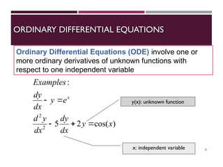
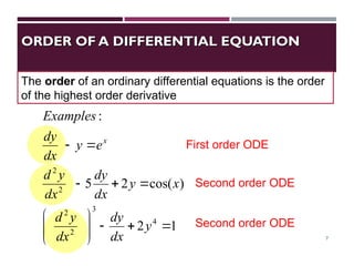
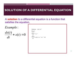
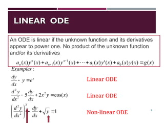
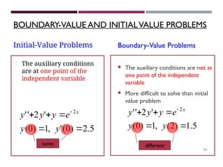
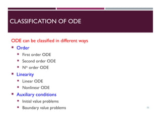
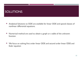
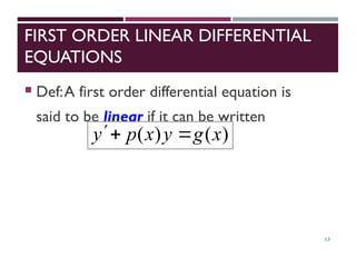
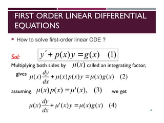
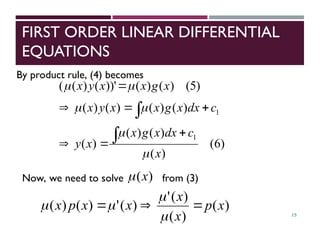
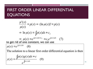
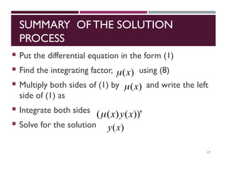
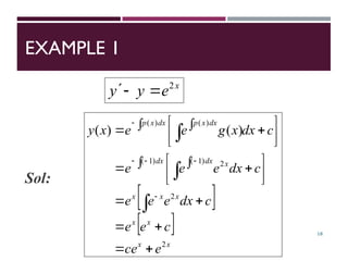
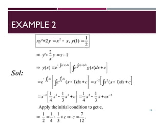
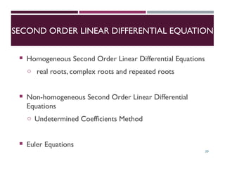
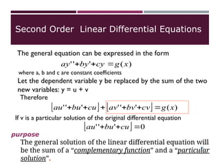
1
Here is Nouman Iftikhar
And I am going to perform the presenation of Ordinary
Differential Equation (ODE) Taught By Honorable
Dr. Saima Mushtaq
Topic : Ordinary Differential Equations
Philip H. Dybvig
2
Reference: Lecture Notes by Paul Dawkins, 2007, page 20-33,
page 102-121,page 137-155 and page 340-344
INTRODUCTION TO ORDINARY
DIFFERENTIAL EQUATIONS (ODE)
 Recall basic definitions of ODE
 Order
 linearity
 initial conditions
 solution
 Classify ODE based on( order, linearity, conditions)
 Classify the solution methods
3
DERIVATIVES
Derivatives
dx
dy
4
Partial Derivatives
u is a function of
more than one
independent variable
Ordinary Derivatives
y is a function of one
independent variable
y
u


DIFFERENTIAL EQUATIONS
Differential
Equations
1
6
2
2

 xy
dx
y
d
5
involve one or more
partial derivatives of
unknown functions
Ordinary Differential Equations
involve one or more
Ordinary derivatives of
unknown functions
0
2
2
2
2






x
u
y
u
Partial Differential Equations
ORDINARY DIFFERENTIAL EQUATIONS
6
)
cos(
2
5
:
2
2
x
y
dx
dy
dx
y
d
e
y
dx
dy
Examples
x





Ordinary Differential Equations (ODE) involve one or
more ordinary derivatives of unknown functions with
respect to one independent variable
y(x): unknown function
x: independent variable
ORDER OF A DIFFERENTIAL EQUATION
7
1
2
)
cos(
2
5
:
4
3
2
2
2
2
















y
dx
dy
dx
y
d
x
y
dx
dy
dx
y
d
e
y
dx
dy
Examples
x
The order of an ordinary differential equations is the order
of the highest order derivative
Second order ODE
First order ODE
Second order ODE
SOLUTION OF A DIFFERENTIAL EQUATION
0
)
(
)
(
)
(
:
Proof
)
(












t
t
t
t
e
e
t
x
dt
t
dx
e
dt
t
dx
e
t
x
Solution
8
A solution to a differential equation is a function that
satisfies the equation.
0
)
(
)
(
:

 t
x
dt
t
dx
Example
LINEAR ODE
LINEAR ODE
9
1
)
cos(
2
5
:
3
2
2
2
2
2
















y
dx
dy
dx
y
d
x
y
x
dx
dy
dx
y
d
e
y
dx
dy
Examples
x
An ODE is linear if the unknown function and its derivatives
appear to power one. No product of the unknown function
and/or its derivatives
Linear ODE
Linear ODE
Non-linear ODE
)
(
)
(
)
(
)
(
'
)
(
)
(
)
(
)
(
)
( 0
1
1
1 x
g
x
y
x
a
x
y
x
a
x
y
x
a
x
y
x
a n
n
n
n 



 
 
BOUNDARY-VALUE AND INITIALVALUE PROBLEMS
Boundary-Value Problems
 The auxiliary conditions are not at
one point of the independent
variable
 More difficult to solve than initial
value problem
5
.
1
)
2
(
,
1
)
0
(
'
2
'
' 2




 
y
y
e
y
y
y x
10
Initial-Value Problems
 The auxiliary conditions
are at one point of the
independent variable
5
.
2
)
0
(
'
,
1
)
0
(
'
2
'
' 2




 
y
y
e
y
y
y x
same different
CLASSIFICATION OF ODE
ODE can be classified in different ways
 Order
 First order ODE
 Second order ODE
 Nth
order ODE
 Linearity
 Linear ODE
 Nonlinear ODE
 Auxiliary conditions
 Initial value problems
 Boundary value problems 11
SOLUTIONS
 Analytical Solutions to ODE are available for linear ODE and special classes of
nonlinear differential equations.
 Numerical method are used to obtain a graph or a table of the unknown
function
 We focus on solving first order linear ODE and second order linear ODE and
Euler equation
12
FIRST ORDER LINEAR DIFFERENTIAL
EQUATIONS
 Def:A first order differential equation is
said to be linear if it can be written
13
)
(
)
( x
g
y
x
p
y 


FIRST ORDER LINEAR DIFFERENTIAL
EQUATIONS
 How to solve first-order linear ODE ?
Sol:
14
)
1
(
)
(
)
( x
g
y
x
p
y 


)
2
(
)
(
)
(
)
(
)
(
)
( x
g
x
y
x
p
x
dx
dy
x 

 

Multiplying both sides by , called an integrating factor,
gives
)
(x

assuming we get
)
3
(
),
(
'
)
(
)
( x
x
p
x 
 
)
4
(
)
(
)
(
)
(
'
)
( x
g
x
y
x
dx
dy
x 

 

FIRST ORDER LINEAR DIFFERENTIAL
EQUATIONS
15
By product rule, (4) becomes
Now, we need to solve from (3)
)
(
)
(
)
(
'
)
(
'
)
(
)
( x
p
x
x
x
x
p
x 






)
6
(
)
(
)
(
)
(
)
(
)
(
)
(
)
(
)
(
)
5
(
)
(
)
(
))'
(
)
(
(
1
1
x
c
dx
x
g
x
x
y
c
dx
x
g
x
x
y
x
x
g
x
x
y
x















)
(x

FIRST ORDER LINEAR DIFFERENTIAL
EQUATIONS
16
)
7
(
)
(
)
(
)
(
ln
)
(
))'
(
(ln
)
(
)
(
)
(
'
)
(
3
)
(
2
2 












dx
x
p
c
dx
x
p
e
c
e
x
c
dx
x
p
x
x
p
x
x
p
x
x





to get rid of one constant, we can use
)
9
(
)
(
)
(
)
(
then
is
equation
al
differenti
order
first
linear
a
o
solution t
The
)
8
(
)
(
)
(
)
(






dx
x
p
dx
x
p
e
c
dx
x
g
x
x
y
e
x


SUMMARY OF THE SOLUTION
PROCESS
 Put the differential equation in the form (1)
 Find the integrating factor, using (8)
 Multiply both sides of (1) by and write the left
side of (1) as
 Integrate both sides
 Solve for the solution
17
)
(x

)
(x

))'
(
)
(
( x
y
x

)
(x
y
EXAMPLE 1
Sol:
18
x
e
y
y 2



 
 
x
x
x
x
x
x
x
x
dx
dx
dx
x
p
dx
x
p
e
ce
c
e
e
c
dx
e
e
e
c
dx
e
e
e
c
dx
x
g
e
e
x
y
2
2
2
)
1
(
)
1
(
)
(
)
(
)
(
)
(











 








 











EXAMPLE 2
Sol:
19
2
1
)
1
(
,
2
' 2



 y
x
x
y
xy
 
.
12
7
3
1
4
1
2
1
c,
get
to
condition
initial
Apply the
3
1
4
1
3
1
4
1
)
1
(
)
1
(
)
(
)
(
1
2
'
2
2
3
4
2
2
2
2
2
)
(
)
(





































 
















c
c
cx
x
x
c
x
x
x
c
dx
x
x
x
c
dx
x
e
e
c
dx
x
g
e
e
x
y
x
y
x
y
dx
x
dx
x
dx
x
p
dx
x
p
SECOND ORDER LINEAR DIFFERENTIAL EQUATIONS
 Homogeneous Second Order Linear Differential Equations
o real roots, complex roots and repeated roots
 Non-homogeneous Second Order Linear Differential
Equations
o Undetermined Coefficients Method
 Euler Equations
20
)
(
'
'
' x
g
cy
by
ay 


where a, b and c are constant coefficients
Let the dependent variable y be replaced by the sum of the two
new variables: y = u + v
Therefore
    )
(
'
'
'
'
'
' x
g
cv
bv
av
cu
bu
au 





If v is a particular solution of the original differential equation
The general solution of the linear differential equation will
be the sum of a “complementary function” and a “particular
solution”.
purpose
Second Order Linear Differential Equations
The general equation can be expressed in the form
  0
'
'
' 

 cu
bu
au
21
0
'
'
' 

 cy
by
ay
Let the solution assumed to be:
rx
e
y 
rx
re
dx
dy
 rx
e
r
dx
y
d 2
2
2

0
)
( 2


 c
br
ar
erx
characteristic equation Real, distinct roots
Double roots
Complex roots
The Complementary Function (solution of the
homogeneous equation)
22
23
x
r
e
y 1
 x
r
e
y 2

x
r
x
r
e
c
e
c
y 2
1
2
1 

Real, Distinct Roots to Characteristic Equation
• Let the roots of the characteristic equation be real, distinct
and of values r1 and r2. Therefore, the solutions of the
characteristic equation are:
• The general solution will be
0
6
'
5
'
' 

 y
y
y 0
6
5
2


 r
r
3
2
2
1


r
r x
x
e
c
e
c
y 3
2
2
1 

• Example
rx
e
y 
rx
rx
rVe
V
e
y 

 '
'
rx
Ve
y 
Let
rx
rx
rx
Ve
r
V
re
V
e
y 2
'
2
'
'
'
'
and 


where V is a
function of x
0
'
'
' 

 cy
by
ay
0
)
(
'
' 
x
V d
cx
V 

rx
rx
rx
rx
xe
c
e
c
e
d
cx
be
y 2
1
)
( 




Equal Roots to Characteristic Equation
• Let the roots of the characteristic equation equal and of value r1 =
r2 = r. Therefore, the solution of the characteristic equation is:
0
c
br
ar2


 0
b
ar
2 

24
)).
sin(
)
(cos(
,
))
sin(
)
(cos(
)
(
2
)
(
1
x
i
x
e
e
y
x
i
x
e
e
y
x
x
i
x
x
i


















).
sin(
cos
:
is
d.e.
the
o
solution t
geneal
the
Therefore,
equation.
al
differenti
the
to
solutions
two
are
and
that
see
easy to
is
It
)
sin(
)
(
2
1
)
(
),
cos(
)
(
2
1
)
(
2
1
2
1
2
1
x
e
c
x)
(
e
c
y(x)
v
u
x
e
y
y
i
x
v
x
e
y
y
x
u
λx
λx
x
x



 









Complex Roots to Characteristic
Equation
Let the roots of the characteristic equation be complex in
the form r1,2 =λ±µi. Therefore, the solution of the
characteristic equation is:
25
(I) Solve 0
9
'
6
'
' 

 y
y
y
characteristic equation
0
9
6
2


 r
r
3
2
1 

r
r
x
e
x
c
c
y 3
2
1 )
( 


Examples
(II) Solve 0
5
'
4
'
' 

 y
y
y
characteristic equation
0
5
4
2


 r
r
i
r 
2
2
,
1
)
sin
cos
( 2
1
2
x
c
x
c
e
y x


26
When g(x) is a polynomial of the form
where all the coefficients are constants. The form of a particular solution is
)
(
'
'
' x
g
cy
by
ay 


c
k
y /

n
n x
a
x
a
x
a
a 


 ...
2
2
1
0
n
n x
x
x
y 


 



 ...
2
2
1
0
Non-homogeneous Differential Equations
(Method of Undetermined Coefficients)
When g(x) is constant, say k, a particular solution of equation is
27
Example
Solve 3
8
4
4
'
4
'
' x
x
y
y
y 



3
2
sx
rx
qx
p
y 



2
3
2
' sx
rx
q
y 


sx
r
y 6
2
'
' 

3
3
2
2
8
4
)
(
4
)
3
2
(
4
)
6
2
( x
x
sx
rx
qx
p
sx
rx
q
sx
r 









equating coefficients of equal powers of x
8
4
0
12
4
4
4
8
6
0
4
4
2









s
s
r
q
r
s
p
q
r
3
2
2
6
10
7 x
x
x
yp 



0
4
4
2


 r
r
characteristic equation
x
c e
x
c
c
y 2
2
1 )
( 

3
2
2
2
1 2
6
10
7
)
( x
x
x
e
x
c
c
y
y
y
x
p
c








0
4
'
4
'
' 

 y
y
y
complementary function
2

r
28
Non-homogeneous Differential Equations
(Method of Undetermined Coefficients)
rx
Ae
y 
• When g(x) is of the form Terx
, where T and r are constants. The
form of a particular solution is
c
br
ar
T
A


 2
• When g(x) is of the form Csinnx + Dcosnx, where C and D are
constants, the form of a particular solution is
nx
F
nx
E
y cos
sin 

2
2
2
2
2
)
(
)
(
b
n
a
n
c
nbD
C
a
n
c
E





2
2
2
2
2
)
(
)
(
b
n
a
n
c
nbD
C
a
n
c
F





29
Example
Solve 18
'
6
'
'
3 
 y
y
Cx
y 
C
y 
'
0
'
' 
y
18
)
C
(
6
)
0
(
3 

3
C 

x
yp 3


0
6
3 2

 r
r
characteristic equation
x
c e
c
c
y 2
2
1 

x
p
c
e
c
c
x
y
y
y
2
2
1
3 





0
'
6
'
'
3 
 y
y
complementary function
2
,
0 2
1 
 r
r
30
Example
Solve
x
e
y
y
y 4
7
8
'
10
'
'
3 



x
Cxe
y 4


x
Ce
x
y 4
)
4
1
(
' 


x
Ce
x
y 4
)
8
16
(
'
' 


7
10
24 

 C
C
2
1


C
x
p xe
y 4
2
1 


0
)
4
)(
2
3
(
8
10
3 2





 r
r
r
r
characteristic equation
x
x
c Be
Ae
y 4
3
/
2 


x
x
x
p
c
Be
Ae
xe
y
y
y
4
3
/
2
4
2
1 







0
8
'
10
'
'
3 

 y
y
y
complementary function
4
,
3
/
2 2
1 

 r
r
31
Example
Solve x
y
y
y 2
cos
52
6
'
'
' 


x
D
x
C
y 2
sin
2
cos 

)
2
cos
2
sin
(
2
' x
D
x
C
y 


)
2
sin
2
cos
(
4
'
' x
D
x
C
y 


0
10
2
52
2
10






D
C
D
C
1
5



D
C
x
x
yp 2
sin
2
cos
5 


0
)
3
)(
2
(
6
2





 r
r
r
r
characteristic equation
x
x
c Be
Ae
y 3
2 


x
x
Be
Ae
y
y
y
x
x
p
c
2
sin
2
cos
5
3
2







0
6
'
'
' 

 y
y
y
complementary function
3
,
2 2
1 

 r
r
32
EULER EQUATIONS
 Def: Euler equations
 Assuming x>0 and all solutions are of the form
y(x) = xr
 Plug into the differential equation to get the
characteristic equation
33
0
'
'
'
2


 cy
bxy
y
ax
.
0
)
(
)
1
( 


 c
r
b
r
ar
SOLVING EULER EQUATIONS: (CASE I)
34
• The characteristic equation has two different real
solutions r1 and r2.
• In this case the functions y = xr1 and y = xr2 are
both solutions to the original equation. The general
solution is: 2
1
2
1
)
( r
r
x
c
x
c
x
y 

.
x
c
x
c
y(x)
.
r
,
r
r-
)
r(r-
y
xy
y
x
3
2
2
5
1
2
1
2
3
2
5
0
15
3
1
2
:
is
equation
stic
characteri
the
,
0
15
'
3
'
'
2













Example:
SOLVING EULER EQUATIONS: (CASE II)
35
• The characteristic equation has two equal roots r1
= r2=r.
• In this case the functions y = xr
and y = xr
lnx are
both solutions to the original equation. The general
solution is: )
ln
(
)
( 2
1 x
c
c
x
x
y r


x.
x
c
x
c
y(x)
.
r
r
)
r(r-
y
xy
y
x
ln
4
0
16
7
1
:
is
equation
stic
characteri
the
,
0
16
'
7
'
'
4
2
4
1
2











Example:
SOLVING EULER EQUATIONS: (CASE III)
36
• The characteristic equation has two complex
roots r1,2 = λ±µi.
x))
(μ
c
x)
(μ
(c
x
y(x)
x
ix
x
x
e
x
λ
x
i
i
ln
sin
ln
cos
:
be
ill
solution w
general
the
roots,
complex
of
case
in the
So,
)
ln
sin(
)
ln
cos(
2
1
ln
)
(




 


 





.
x
x
c
x
x
c
y(x)
i.
r
r
)
r(r-
y
xy
y
x
)
ln
3
sin(
)
ln
3
cos(
3
1
0
4
3
1
:
is
equation
stic
characteri
the
,
0
4
'
3
'
'
1
2
1
1
2
,
1
2















Example:

Ordinary differential equation Presentation

  • 1.
    1 Here is NoumanIftikhar And I am going to perform the presenation of Ordinary Differential Equation (ODE) Taught By Honorable Dr. Saima Mushtaq
  • 2.
    Topic : OrdinaryDifferential Equations Philip H. Dybvig 2 Reference: Lecture Notes by Paul Dawkins, 2007, page 20-33, page 102-121,page 137-155 and page 340-344
  • 3.
    INTRODUCTION TO ORDINARY DIFFERENTIALEQUATIONS (ODE)  Recall basic definitions of ODE  Order  linearity  initial conditions  solution  Classify ODE based on( order, linearity, conditions)  Classify the solution methods 3
  • 4.
    DERIVATIVES Derivatives dx dy 4 Partial Derivatives u isa function of more than one independent variable Ordinary Derivatives y is a function of one independent variable y u  
  • 5.
    DIFFERENTIAL EQUATIONS Differential Equations 1 6 2 2   xy dx y d 5 involveone or more partial derivatives of unknown functions Ordinary Differential Equations involve one or more Ordinary derivatives of unknown functions 0 2 2 2 2       x u y u Partial Differential Equations
  • 6.
    ORDINARY DIFFERENTIAL EQUATIONS ORDINARYDIFFERENTIAL EQUATIONS 6 ) cos( 2 5 : 2 2 x y dx dy dx y d e y dx dy Examples x      Ordinary Differential Equations (ODE) involve one or more ordinary derivatives of unknown functions with respect to one independent variable y(x): unknown function x: independent variable
  • 7.
    ORDER OF ADIFFERENTIAL EQUATION ORDER OF A DIFFERENTIAL EQUATION 7 1 2 ) cos( 2 5 : 4 3 2 2 2 2                 y dx dy dx y d x y dx dy dx y d e y dx dy Examples x The order of an ordinary differential equations is the order of the highest order derivative Second order ODE First order ODE Second order ODE
  • 8.
    SOLUTION OF ADIFFERENTIAL EQUATION SOLUTION OF A DIFFERENTIAL EQUATION 0 ) ( ) ( ) ( : Proof ) (             t t t t e e t x dt t dx e dt t dx e t x Solution 8 A solution to a differential equation is a function that satisfies the equation. 0 ) ( ) ( :   t x dt t dx Example
  • 9.
    LINEAR ODE LINEAR ODE 9 1 ) cos( 2 5 : 3 2 2 2 2 2                 y dx dy dx y d x y x dx dy dx y d e y dx dy Examples x AnODE is linear if the unknown function and its derivatives appear to power one. No product of the unknown function and/or its derivatives Linear ODE Linear ODE Non-linear ODE ) ( ) ( ) ( ) ( ' ) ( ) ( ) ( ) ( ) ( 0 1 1 1 x g x y x a x y x a x y x a x y x a n n n n        
  • 10.
    BOUNDARY-VALUE AND INITIALVALUEPROBLEMS Boundary-Value Problems  The auxiliary conditions are not at one point of the independent variable  More difficult to solve than initial value problem 5 . 1 ) 2 ( , 1 ) 0 ( ' 2 ' ' 2       y y e y y y x 10 Initial-Value Problems  The auxiliary conditions are at one point of the independent variable 5 . 2 ) 0 ( ' , 1 ) 0 ( ' 2 ' ' 2       y y e y y y x same different
  • 11.
    CLASSIFICATION OF ODE ODEcan be classified in different ways  Order  First order ODE  Second order ODE  Nth order ODE  Linearity  Linear ODE  Nonlinear ODE  Auxiliary conditions  Initial value problems  Boundary value problems 11
  • 12.
    SOLUTIONS  Analytical Solutionsto ODE are available for linear ODE and special classes of nonlinear differential equations.  Numerical method are used to obtain a graph or a table of the unknown function  We focus on solving first order linear ODE and second order linear ODE and Euler equation 12
  • 13.
    FIRST ORDER LINEARDIFFERENTIAL EQUATIONS  Def:A first order differential equation is said to be linear if it can be written 13 ) ( ) ( x g y x p y   
  • 14.
    FIRST ORDER LINEARDIFFERENTIAL EQUATIONS  How to solve first-order linear ODE ? Sol: 14 ) 1 ( ) ( ) ( x g y x p y    ) 2 ( ) ( ) ( ) ( ) ( ) ( x g x y x p x dx dy x      Multiplying both sides by , called an integrating factor, gives ) (x  assuming we get ) 3 ( ), ( ' ) ( ) ( x x p x    ) 4 ( ) ( ) ( ) ( ' ) ( x g x y x dx dy x     
  • 15.
    FIRST ORDER LINEARDIFFERENTIAL EQUATIONS 15 By product rule, (4) becomes Now, we need to solve from (3) ) ( ) ( ) ( ' ) ( ' ) ( ) ( x p x x x x p x        ) 6 ( ) ( ) ( ) ( ) ( ) ( ) ( ) ( ) ( ) 5 ( ) ( ) ( ))' ( ) ( ( 1 1 x c dx x g x x y c dx x g x x y x x g x x y x                ) (x 
  • 16.
    FIRST ORDER LINEARDIFFERENTIAL EQUATIONS 16 ) 7 ( ) ( ) ( ) ( ln ) ( ))' ( (ln ) ( ) ( ) ( ' ) ( 3 ) ( 2 2              dx x p c dx x p e c e x c dx x p x x p x x p x x      to get rid of one constant, we can use ) 9 ( ) ( ) ( ) ( then is equation al differenti order first linear a o solution t The ) 8 ( ) ( ) ( ) (       dx x p dx x p e c dx x g x x y e x  
  • 17.
    SUMMARY OF THESOLUTION PROCESS  Put the differential equation in the form (1)  Find the integrating factor, using (8)  Multiply both sides of (1) by and write the left side of (1) as  Integrate both sides  Solve for the solution 17 ) (x  ) (x  ))' ( ) ( ( x y x  ) (x y
  • 18.
    EXAMPLE 1 Sol: 18 x e y y 2       x x x x x x x x dx dx dx x p dx x p e ce c e e c dx e e e c dx e e e c dx x g e e x y 2 2 2 ) 1 ( ) 1 ( ) ( ) ( ) ( ) (                                  
  • 19.
    EXAMPLE 2 Sol: 19 2 1 ) 1 ( , 2 ' 2    y x x y xy   . 12 7 3 1 4 1 2 1 c, get to condition initial Apply the 3 1 4 1 3 1 4 1 ) 1 ( ) 1 ( ) ( ) ( 1 2 ' 2 2 3 4 2 2 2 2 2 ) ( ) (                                                        c c cx x x c x x x c dx x x x c dx x e e c dx x g e e x y x y x y dx x dx x dx x p dx x p
  • 20.
    SECOND ORDER LINEARDIFFERENTIAL EQUATIONS  Homogeneous Second Order Linear Differential Equations o real roots, complex roots and repeated roots  Non-homogeneous Second Order Linear Differential Equations o Undetermined Coefficients Method  Euler Equations 20
  • 21.
    ) ( ' ' ' x g cy by ay    wherea, b and c are constant coefficients Let the dependent variable y be replaced by the sum of the two new variables: y = u + v Therefore     ) ( ' ' ' ' ' ' x g cv bv av cu bu au       If v is a particular solution of the original differential equation The general solution of the linear differential equation will be the sum of a “complementary function” and a “particular solution”. purpose Second Order Linear Differential Equations The general equation can be expressed in the form   0 ' ' '    cu bu au 21
  • 22.
    0 ' ' '    cy by ay Letthe solution assumed to be: rx e y  rx re dx dy  rx e r dx y d 2 2 2  0 ) ( 2    c br ar erx characteristic equation Real, distinct roots Double roots Complex roots The Complementary Function (solution of the homogeneous equation) 22
  • 23.
    23 x r e y 1  x r e y2  x r x r e c e c y 2 1 2 1   Real, Distinct Roots to Characteristic Equation • Let the roots of the characteristic equation be real, distinct and of values r1 and r2. Therefore, the solutions of the characteristic equation are: • The general solution will be 0 6 ' 5 ' '    y y y 0 6 5 2    r r 3 2 2 1   r r x x e c e c y 3 2 2 1   • Example
  • 24.
    rx e y  rx rx rVe V e y   ' ' rx Ve y  Let rx rx rx Ve r V re V e y 2 ' 2 ' ' ' ' and    where V is a function of x 0 ' ' '    cy by ay 0 ) ( ' '  x V d cx V   rx rx rx rx xe c e c e d cx be y 2 1 ) (      Equal Roots to Characteristic Equation • Let the roots of the characteristic equation equal and of value r1 = r2 = r. Therefore, the solution of the characteristic equation is: 0 c br ar2    0 b ar 2   24
  • 25.
  • 26.
    (I) Solve 0 9 ' 6 ' '   y y y characteristic equation 0 9 6 2    r r 3 2 1   r r x e x c c y 3 2 1 ) (    Examples (II) Solve 0 5 ' 4 ' '    y y y characteristic equation 0 5 4 2    r r i r  2 2 , 1 ) sin cos ( 2 1 2 x c x c e y x   26
  • 27.
    When g(x) isa polynomial of the form where all the coefficients are constants. The form of a particular solution is ) ( ' ' ' x g cy by ay    c k y /  n n x a x a x a a     ... 2 2 1 0 n n x x x y          ... 2 2 1 0 Non-homogeneous Differential Equations (Method of Undetermined Coefficients) When g(x) is constant, say k, a particular solution of equation is 27
  • 28.
    Example Solve 3 8 4 4 ' 4 ' ' x x y y y    3 2 sx rx qx p y     2 3 2 ' sx rx q y    sx r y 6 2 ' '   3 3 2 2 8 4 ) ( 4 ) 3 2 ( 4 ) 6 2 ( x x sx rx qx p sx rx q sx r           equating coefficients of equal powers of x 8 4 0 12 4 4 4 8 6 0 4 4 2          s s r q r s p q r 3 2 2 6 10 7 x x x yp     0 4 4 2    r r characteristic equation x c e x c c y 2 2 1 ) (   3 2 2 2 1 2 6 10 7 ) ( x x x e x c c y y y x p c         0 4 ' 4 ' '    y y y complementary function 2  r 28
  • 29.
    Non-homogeneous Differential Equations (Methodof Undetermined Coefficients) rx Ae y  • When g(x) is of the form Terx , where T and r are constants. The form of a particular solution is c br ar T A    2 • When g(x) is of the form Csinnx + Dcosnx, where C and D are constants, the form of a particular solution is nx F nx E y cos sin   2 2 2 2 2 ) ( ) ( b n a n c nbD C a n c E      2 2 2 2 2 ) ( ) ( b n a n c nbD C a n c F      29
  • 30.
    Example Solve 18 ' 6 ' ' 3  y y Cx y  C y  ' 0 ' '  y 18 ) C ( 6 ) 0 ( 3   3 C   x yp 3   0 6 3 2   r r characteristic equation x c e c c y 2 2 1   x p c e c c x y y y 2 2 1 3       0 ' 6 ' ' 3   y y complementary function 2 , 0 2 1   r r 30
  • 31.
    Example Solve x e y y y 4 7 8 ' 10 ' ' 3     x Cxe y4   x Ce x y 4 ) 4 1 ( '    x Ce x y 4 ) 8 16 ( ' '    7 10 24    C C 2 1   C x p xe y 4 2 1    0 ) 4 )( 2 3 ( 8 10 3 2       r r r r characteristic equation x x c Be Ae y 4 3 / 2    x x x p c Be Ae xe y y y 4 3 / 2 4 2 1         0 8 ' 10 ' ' 3    y y y complementary function 4 , 3 / 2 2 1    r r 31
  • 32.
    Example Solve x y y y 2 cos 52 6 ' ' '   x D x C y 2 sin 2 cos   ) 2 cos 2 sin ( 2 ' x D x C y    ) 2 sin 2 cos ( 4 ' ' x D x C y    0 10 2 52 2 10       D C D C 1 5    D C x x yp 2 sin 2 cos 5    0 ) 3 )( 2 ( 6 2       r r r r characteristic equation x x c Be Ae y 3 2    x x Be Ae y y y x x p c 2 sin 2 cos 5 3 2        0 6 ' ' '    y y y complementary function 3 , 2 2 1    r r 32
  • 33.
    EULER EQUATIONS  Def:Euler equations  Assuming x>0 and all solutions are of the form y(x) = xr  Plug into the differential equation to get the characteristic equation 33 0 ' ' ' 2    cy bxy y ax . 0 ) ( ) 1 (     c r b r ar
  • 34.
    SOLVING EULER EQUATIONS:(CASE I) 34 • The characteristic equation has two different real solutions r1 and r2. • In this case the functions y = xr1 and y = xr2 are both solutions to the original equation. The general solution is: 2 1 2 1 ) ( r r x c x c x y   . x c x c y(x) . r , r r- ) r(r- y xy y x 3 2 2 5 1 2 1 2 3 2 5 0 15 3 1 2 : is equation stic characteri the , 0 15 ' 3 ' ' 2              Example:
  • 35.
    SOLVING EULER EQUATIONS:(CASE II) 35 • The characteristic equation has two equal roots r1 = r2=r. • In this case the functions y = xr and y = xr lnx are both solutions to the original equation. The general solution is: ) ln ( ) ( 2 1 x c c x x y r   x. x c x c y(x) . r r ) r(r- y xy y x ln 4 0 16 7 1 : is equation stic characteri the , 0 16 ' 7 ' ' 4 2 4 1 2            Example:
  • 36.
    SOLVING EULER EQUATIONS:(CASE III) 36 • The characteristic equation has two complex roots r1,2 = λ±µi. x)) (μ c x) (μ (c x y(x) x ix x x e x λ x i i ln sin ln cos : be ill solution w general the roots, complex of case in the So, ) ln sin( ) ln cos( 2 1 ln ) (                . x x c x x c y(x) i. r r ) r(r- y xy y x ) ln 3 sin( ) ln 3 cos( 3 1 0 4 3 1 : is equation stic characteri the , 0 4 ' 3 ' ' 1 2 1 1 2 , 1 2                Example: