Downloaded 10 times


![(n-1) +
(n-1)
=
It will be sensitive to steep slopes & large amplitudes provided the wavelength
(n) + is different from those encountered during adaptation. In this way clipping the
prediction error provides us with the desired splitting of the signal into a quasi-
stationary part (below threshold) and local non-stationaries(above threshold).
However, experience has shown that criterion given by Eq. 4.105 with a
threshold setting suitable for segmantation is far too sensitive for transient
detection. EEG spikes generally have a duration of 50-100 ms. As a reasonable
method for the elimination o ffalse alarm caused by random fluctuations in the
prediction error it is the elimination of false alarm caused by random
fluctuations in the prediction error power with this time constant. Accordingly,
the following heuristic criterion is adopted as suggested in [1], i.e.
= (n-1)+
Page 9](https://image.slidesharecdn.com/bspppt-130319122524-phpapp02/75/Bsp-ppt-9-2048.jpg)
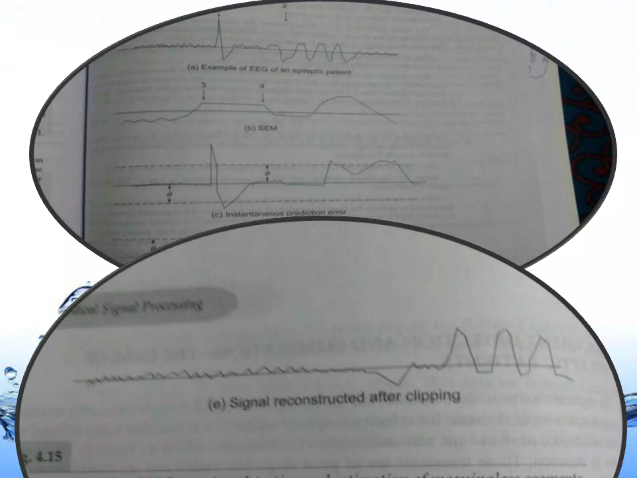
![For a demonstration of the detection of spikes in real life situations using the
above procedure we refer to the example discussed in [1] and given in detail in
Fig. 4.16.
Page 11](https://image.slidesharecdn.com/bspppt-130319122524-phpapp02/75/Bsp-ppt-11-2048.jpg)
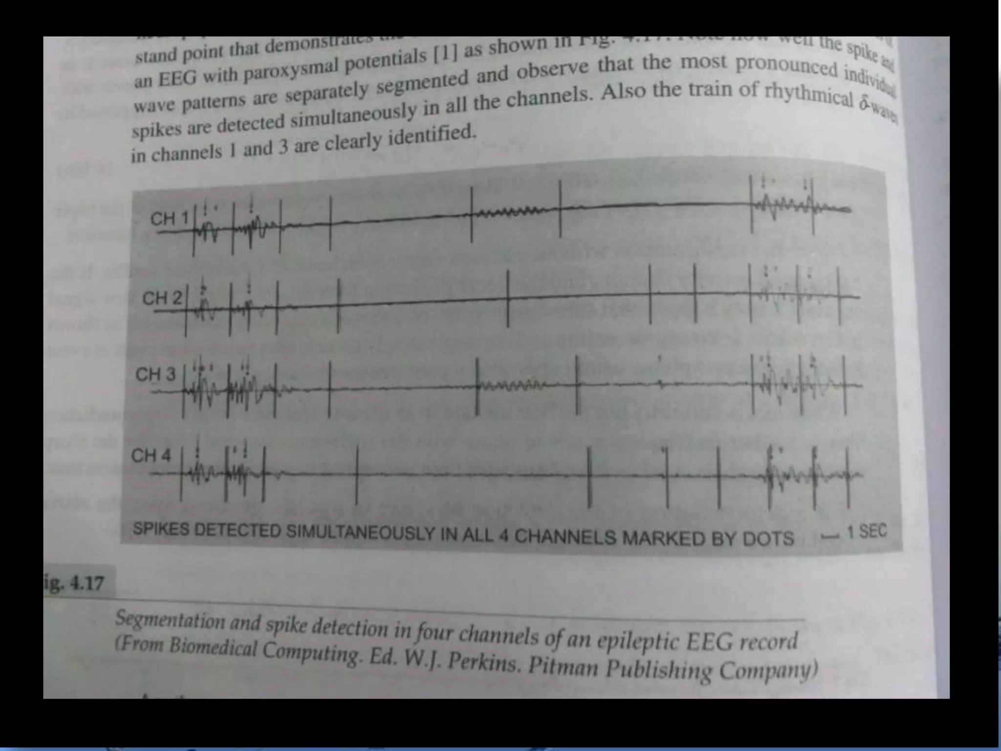
![OVERALL PERFORMANCE
The only real way to find out would be to construct the entire algorithm
which takes the EEG as input & produces a diagnosis, say healthy or
sick, as output and then compare it with that given by the neurophysiologist.
Nevertheless, we give an example, the most interesting, from a clinical
stand point that demonstrates the effectiveness of the proposed method on
four channels of an EEG with paroxysmal potentials[1] as shown in Fig.
4.17. Note how well the spike and wave patterns are separately segmented
and observe that the most pronounced individual spikes are detected
simultaneously in all the channels. Also the train of rhythmical delta waves
in channels 1 and 3 are clearly identified.
Page 12](https://image.slidesharecdn.com/bspppt-130319122524-phpapp02/75/Bsp-ppt-12-2048.jpg)
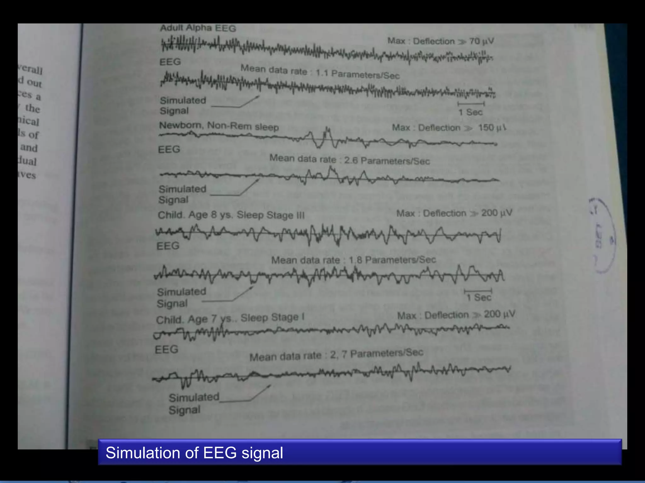


The document discusses EEG signal segmentation and transient detection techniques. It proposes using linear prediction filters to model EEG signals as quasi-stationary segments. Transients are detected as outliers from the prediction error signal above a threshold. The technique clips prediction errors to remove transient influence on segmentation. It demonstrates effective segmentation of spike and wave patterns from multi-channel EEGs. Performance is judged by reconstructing EEGs from estimated filters and comparing to original signals.