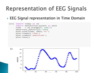
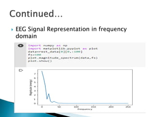
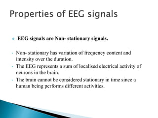
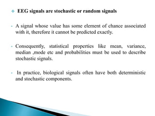
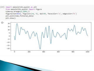
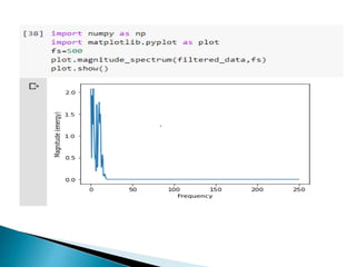
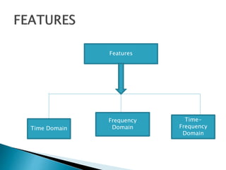
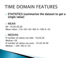
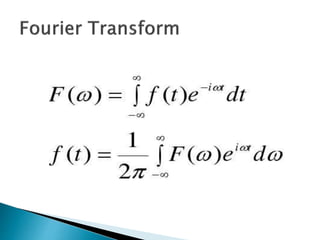
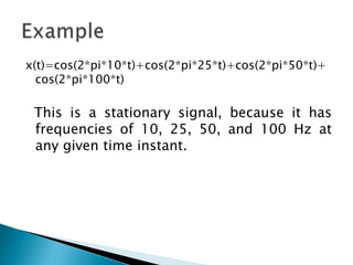
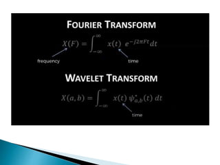
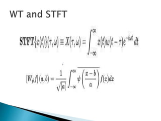
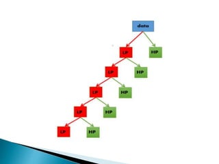
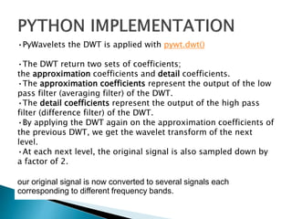
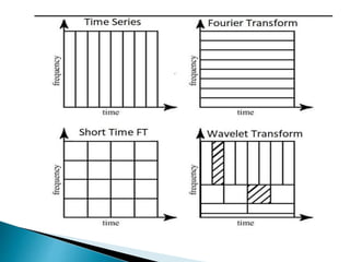
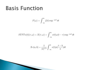
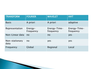
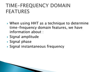
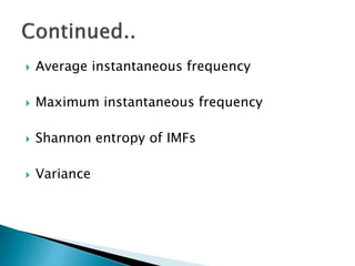
 An EEG is a test that detects abnormalities in your brain
waves, or in the electrical activity of your brain
 Non-invasive with electrodes being placed on the scalp.
 EEG refers to recording of brain spontaneous electrical
activity over a period of time.
 The brain consists of billion of cells ,half of which are
neurons, half of which help and facilitate the activity of
neurons.
 Whenever any activity occurs it generates electrical impulse in
the brain due to which thousands of neurons fire in sync, and
electric field is generated and it is measured with the help of
electrodes.
 EEG monitors the time course of electrical activity generated
by brain, so interpreting EEG depending on the areas of
cortex:
 Occipital cortex:
• Responsible for processing of visual information.
• EEG experiments with visual stimulus (video , images).
 Parietal cortex:
• Responsible for motor functions and active during self
referential tasks.
 Temporal cortex:
• Responsible for language processing and speech production.
 Frontal cortex:
• Responsible for control and monitor our behavior.
 The EEG is described in terms of :
1. Rhythmic activity : It is divided into bands of frequency
and frequency bands are extracted using methods like
Fourier transforms, STFT, DWT,HHT and Filters etc.
Plot of different freq. bands computed on stress dataset
 Dominates when a person tries to combine two different senses such as sound
and sight.
 These are involved in higher processing tasks as well as cognitive functioning.
 It has been found that individuals who are mentally challenged and have
learning disabilities tend to have lower gamma activity than average.
Wave Relation with Activities
 Too much: Anxiety, high arousal, stress
 Too little: Depression, learning disabilities
 Optimal: Binding senses, cognition, information processing, learning,
perception, Rapid Eye Movement.
 Increase gamma waves: Meditation
 EEG Signal representation in Time Domain
 EEG Signal Representation in frequency
domain
 EEG signals are Non- stationary signals.
• Non- stationary has variation of frequency content and
intensity over the duration.
• The EEG represents a sum of localised electrical activity of
neurons in the brain.
• The brain cannot be considered stationary in time since a
human being performs different activities.
 EEG signals are stochastic or random signals
• A signal whose value has some element of chance associated
with it, therefore it cannot be predicted exactly.
• Consequently, statistical properties like mean, variance,
median ,mode etc and probabilities must be used to describe
stochastic signals.
• In practice, biological signals often have both deterministic
and stochastic components.
 EEG signals are easily contaminated by noise also known as
artefacts which occur mainly due to activities which are not
occurring in brain.
 Some of the most common artefacts are listed below:
◦ EOG or Eye-induced artifacts (includes eye blinks, eye movements and
extra-ocular muscle activity)
◦ ECG (cardiac) artifacts
◦ EMG (muscle activation)-induced artifacts
◦ 50Hz/60Hz line interference
 1) Filtering
Types of Filters:
◦ Low pass
◦ High-pass
◦ Bandpass
◦ Band-stop
◦ Notch Filter
Ideal Filters
Practical Filters
 Lets say we an input given as
 x(t) = 𝑒 𝑗2𝑡
+ 𝑒 𝑗4𝑡
+ 𝑒 𝑗8𝑡
+𝑒−𝑗2𝑡
+ 𝑒−𝑗4𝑡
where 2,4,8 are the frequencies present in the
signal.

H(w)
Impulse ResponseX(t) Y(t)
Features
Time Domain
Frequency
Domain
Time-
Frequency
Domain
 STATISTICS (summarize the dataset to get a
single value)
 MEAN
EX- 10,20,30,50
Mean value= (10+20+30+40)/4=100/4=25
 MEDIAN
If number of values are odd : 10,20,30
Median=20
If number of values are even : 10 20 30 40
Median = (20+30)/2=25
 MODE
Ex- 10,20,30,20,40,20,50,20
Mode- 20
 Time Domain Features:
 Mean, standard deviation, variance
 First difference
 Normalized first difference
 Second difference
 Normalized second difference
 Hjorth Features
x(t)=cos(2*pi*10*t)+cos(2*pi*25*t)+cos(2*pi*50*t)+
cos(2*pi*100*t)
This is a stationary signal, because it has
frequencies of 10, 25, 50, and 100 Hz at
any given time instant.
 Consider a Non-stationary signal with four
different frequency components at four
different time intervals. The interval 0 to 300
ms has a 100 Hz sinusoid, the interval 300 to
600 ms has a 50 Hz sinusoid, the interval
600 to 800 ms has a 25 Hz sinusoid, and
finally the interval 800 to 1000 ms has a 10
Hz sinusoid.
 FT of both of previous signals show four
spectral components at exactly the same
frequencies, i.e., at 10, 25, 50, and 100 Hz.
Other than the ripples, and the difference in
amplitude (which can always be normalized),
the two spectrums are almost identical,
although the corresponding time-domain
signals are not even close to each other. Both
of the signals involve the same frequency
components, but the first one has these
frequencies at all times, the second one has
these frequencies at different intervals.
 For practical purposes it is difficult to make the
separation, since there are a lot of practical
stationary signals, as well as non-stationary
ones.
 Almost all biological signals, for example, are
non-stationary.
 Some of the most famous ones are ECG (electrical
activity of the heart, electrocardiograph), EEG
(electrical activity of the brain,
electroencephalograph), and EMG (electrical
activity of the muscles, electromyogram).
 In STFT, the non-stationary signal is divided into small
enough segments, where these segments (portions) of
the signal can be assumed to be stationary.
 For this purpose, a window function "w" is chosen. The
width of this window must be equal to the segment of
the signal where its stationarity is valid.
 This window function is first located to the very
beginning of signal. That is, the window function is
located at t = 0. Let's suppose that the width of the
window is "T" s. At this time instant (t = 0), the window
function will overlap with the first T/2 seconds ( It is
assumed that all time units are in seconds).
 The window function and the signal are then
multiplied. By doing this, only the first T/2 seconds
of the signal is being chosen, with the appropriate
weighting of the window (if the window is a
rectangle, with amplitude "1", then the product will
be equal to the signal). Then this product is
assumed to be just another signal, whose FT is to
be taken. In other words, FT of this product is
taken, just as taking the FT of any signal.
 The result of this transformation is the FT of the
first T/2 seconds of the signal. If this portion of the
signal is stationary, as it is assumed, then there will
be no problem and the obtained result will be a
true frequency representation of the first T/2
seconds of the signal.
 The next step, would be shifting this window
(for some t1 seconds) to a new location,
multiplying with the signal, and taking the FT
of the product. This procedure is followed,
until the end of the signal is reached by
shifting the window with "t1" seconds
intervals.
 Heisenberg Uncertainty Principle: one cannot
know what spectral components exist at what
instances of times. What one can know are the
time intervals in which certain band of
frequencies exist, which is a resolution
problem.
 The problem with the STFT has something to
do with the width of the window function that
is used. To be technically correct, this width of
the window function is known as the support of
the window. If the window function is narrow,
than it is known as compactly supported.
 In the FT there is no resolution problem in the
frequency domain, i.e., we know exactly what
frequencies exist; similarly we there is no time
resolution problem in the time domain, since
we know the value of the signal at every instant
of time. Conversely, the time resolution in the
FT, and the frequency resolution in the time
domain are zero, since we have no information
about them.
 What gives the perfect frequency resolution in
the FT is the fact that the window used in the
FT is its kernel, the exp{jwt} function, which
lasts at all times from minus infinity to plus
infinity and the kernel itself is a window of
infinite length.
 In STFT, our window is of finite length, thus
it covers only a portion of the signal, which
causes the frequency resolution to get
poorer. We no longer know the exact
frequency components that exist in the
signal, but we only know a band of
frequencies that exist.
 If length of the window in the STFT is
selected as infinite, just like as it is in the
FT, to get perfect frequency resolution, than
we loose all the time information. In this
case, we basically end up with the FT
instead of STFT.
Narrow window ===>good time resolution,
poor frequency resolution
Wide-window===> good frequency
resolution, poor time resolution
 FREQUENCY DOMAIN FEATURES
• Power spectral density (psd)
• Spectral Entropy
• Band Power
• Relative Power
 Starting with the drawbacks of FT and STFT:
 FT is localized in frequency ie., it does not
give any information about the time.
 It is not able to differentiate between
stationary and non-stationary signals.
 STFT although it works on both stationary
and non-stationary signals, it still does not
have good resolution as the width of window
is fixed.
Narrow window ===>good time resolution, poor frequency resolution
Wide-window===> good frequency resolution, poor time resolution
 f,t,zxx=scipy.signal.stft(x,fs,window='hann',n
perseg=5)
 Wavelets are functions that “wave” above and
below the x-axis, have
◦ varying frequency,
◦ limited duration, and
◦ an average value of zero
This is in contrast to FT, which represent a signal in
terms of sinusoids. FT provides a signal which is
localized only in the frequency domain.
 WT provides the time-frequency
representation.
 Often times a particular spectral component
occurring at any instant can be of particular
interest.
 For example, in EEGs, the latency of an event-
related potential is of particular interest
(Event-related potential is the response of the
brain to a specific stimulus like flash-light,
the latency of this response is the amount of
time elapsed between the onset of the
stimulus and the response).
 Each wavelet is characterized by scaling
parameter ‘a’ and translation parameter ‘b’.
 It works well for non-linear , discontinuous
and non-stationary signals.
 It is highly suited to represent the natural
signals like EEG,ECG etc.
WT
CWT DWT
 The continuous wavelet transform of a
function f(t) (assumed to have zero mean and
finite energy) C(τ,s ) is defined as convolution
Translation
Parameter,
(measure of time)
Scale Parameter
(measure of
frequency)
Normalization constant
Mother wavelet (window)
 The integral measures the comparison of the
local shape of the signal and the shape of the
wavelet.
 By changing the value of the dilation factor s,
one can zoom in and out of the signal.
 Localization in time is achieved by selecting
τ.
 Take a wavelet and compare it to a section
at the start of the original signal.
 Calculate a number, C, that represents how
closely correlated the wavelet is with this
section of the signal. The higher C is, the
more the similarity.
 Shift the wavelet to the right and repeat
steps 1 and 2 until you've covered the
whole signal.
 Scale the wavelet and repeat steps 1
through 3.
 In practice, the DWT is always
implemented as a filter-bank.
 This means that it is implemented as a
cascade of high-pass and low-pass filters.
 This is because filter banks are a very
efficient way of splitting a signal of into
several frequency sub-bands.
 To apply the DWT on a signal, we start with the
smallest scale. As we have seen before, small
scales correspond with high frequencies. This
means that we first analyze high frequency
behavior.
 At the second stage, the scale increases with a
factor of two (the frequency decreases with a
factor of two), and we are analyzing behavior
around half of the maximum frequency.
 At the third stage, the scale factor is four and we
are analyzing frequency behavior around a
quarter of the maximum frequency. And this
goes on and on, until we have reached the
maximum decomposition level.
 To understand this we should also know that
at each subsequent stage the number of
samples in the signal is reduced with a factor
of two.
 Due to this down-sampling, at some stage in
the process the number of samples in our
signal will become smaller than the length of
the wavelet filter and we will have reached the
maximum decomposition level.
 To give an example, suppose we have a signal
with frequencies up to 1000 Hz. In the first stage
we split our signal into a low-frequency part and
a high-frequency part, i.e. 0-500 Hz and 500-
1000 Hz.
At the second stage we take the low-frequency
part and again split it into two parts: 0-250 Hz and
250-500 Hz.
At the third stage we split the 0-250 Hz part into a
0-125 Hz part and a 125-250 Hz part.
This goes on until we have reached the level of
refinement we need or until we run out of samples.
•PyWavelets the DWT is applied with pywt.dwt()
•The DWT return two sets of coefficients;
the approximation coefficients and detail coefficients.
•The approximation coefficients represent the output of the low
pass filter (averaging filter) of the DWT.
•The detail coefficients represent the output of the high pass
filter (difference filter) of the DWT.
•By applying the DWT again on the approximation coefficients of
the previous DWT, we get the wavelet transform of the next
level.
•At each next level, the original signal is also sampled down by
a factor of 2.
our original signal is now converted to several signals each
corresponding to different frequency bands.
 So far we have looked into:
◦ Fourier Transform
◦ Short Time Fourier Transform
◦ Wavelet Transform
 All these transforms have a common feature
that the basis function is fixed a priori. They
do-not belong to the class of Adaptive
Transforms
 All these transforms have strong
mathematical background.
 HHT is a two step process
1) Empirical Mode Decomposition
2) Hilbert Spectral Analysis
.
The Hilbert–Huang transform (HHT) is a way to decompose a signal into
so-called intrinsic mode functions (IMF) along with a trend, and
obtain instantaneous frequency data.
It is designed to work well for data that is :
• Non-stationary
• Non-linear.
In contrast to other common transforms like the Fourier transform, the
HHT is more like an algorithm (an empirical approach) that can be
applied to a data set, rather than a theoretical tool
 Empirical Mode Decomposition (EMD)
separates a signal in several Intrinsic Mode
Functions (IMFs).
 IMFs satisfy the following criteria:
1) In the whole data set, the number of extrema and
the number of zero-crossings must either be equal or
differ at most by one.
2) At any point, the mean value of the envelope
defined by the local maxima and the envelope
defined by the local minima is zero.
 Find the local extrema of x(t).
 Find the maximum envelope e+(t) of x(t) by
fitting a natural cubic spline through the local
maxima.
 Then, repeat this step to find the minimum
envelope, e−(t), by using the local minima.
 3) Compute an approximation to the local
average:
m(t) = (e+(t) + e−(t))/2
 Find the proto-mode function:
pi(t) = x(t)- m(t)
Check if pi(t) is an IMF.
The properties for a signal to be considered as
an IMF are given below.
a. The number of extrema and the number of
zero crossings may differ by no more than
one.
b. The local average is zero.
 If pi(t) is not an IMF, repeat the EMD sifting
process by setting:
x(t) = pi(t)
 Else, IMFi(t) = pi(t)
 In this equation, cj are IMFs and rn is the
residue.
 This algorithm stops when residue becomes
so small that no IMFs can be obtained.
 Having obtained the intrinsic mode function
components, the instantaneous
frequency can be computed using the Hilbert
transform.
 As a result HHT gives information of
instantaneous variation in magnitude and
frequency of the IMF with respect to time.
TRANSFORM FOURIER WAVELET HHT
Basis A priori A priori adaptive
Representation Energy-
Frequency
Energy-Time-
frequency
Energy-Time-
frequency
Non-Linear data no no yes
Non-stationary
data
no yes yes
Frequency Global Regional Local
 When using HHT as a technique to determine
time-frequency domain features, we have
information about :
 Signal amplitude
 Signal phase
 Signal instantaneous frequency
 Average instantaneous frequency
 Maximum instantaneous frequency
 Shannon entropy of IMFs
 Variance

EEG Signal processing

  • 2.
     An EEGis a test that detects abnormalities in your brain waves, or in the electrical activity of your brain  Non-invasive with electrodes being placed on the scalp.  EEG refers to recording of brain spontaneous electrical activity over a period of time.
  • 3.
     The brainconsists of billion of cells ,half of which are neurons, half of which help and facilitate the activity of neurons.  Whenever any activity occurs it generates electrical impulse in the brain due to which thousands of neurons fire in sync, and electric field is generated and it is measured with the help of electrodes.
  • 4.
     EEG monitorsthe time course of electrical activity generated by brain, so interpreting EEG depending on the areas of cortex:  Occipital cortex: • Responsible for processing of visual information. • EEG experiments with visual stimulus (video , images).
  • 5.
     Parietal cortex: •Responsible for motor functions and active during self referential tasks.  Temporal cortex: • Responsible for language processing and speech production.  Frontal cortex: • Responsible for control and monitor our behavior.
  • 6.
     The EEGis described in terms of : 1. Rhythmic activity : It is divided into bands of frequency and frequency bands are extracted using methods like Fourier transforms, STFT, DWT,HHT and Filters etc.
  • 8.
    Plot of differentfreq. bands computed on stress dataset
  • 9.
     Dominates whena person tries to combine two different senses such as sound and sight.  These are involved in higher processing tasks as well as cognitive functioning.  It has been found that individuals who are mentally challenged and have learning disabilities tend to have lower gamma activity than average. Wave Relation with Activities  Too much: Anxiety, high arousal, stress  Too little: Depression, learning disabilities  Optimal: Binding senses, cognition, information processing, learning, perception, Rapid Eye Movement.  Increase gamma waves: Meditation
  • 12.
     EEG Signalrepresentation in Time Domain
  • 13.
     EEG SignalRepresentation in frequency domain
  • 14.
     EEG signalsare Non- stationary signals. • Non- stationary has variation of frequency content and intensity over the duration. • The EEG represents a sum of localised electrical activity of neurons in the brain. • The brain cannot be considered stationary in time since a human being performs different activities.
  • 15.
     EEG signalsare stochastic or random signals • A signal whose value has some element of chance associated with it, therefore it cannot be predicted exactly. • Consequently, statistical properties like mean, variance, median ,mode etc and probabilities must be used to describe stochastic signals. • In practice, biological signals often have both deterministic and stochastic components.
  • 16.
     EEG signalsare easily contaminated by noise also known as artefacts which occur mainly due to activities which are not occurring in brain.  Some of the most common artefacts are listed below: ◦ EOG or Eye-induced artifacts (includes eye blinks, eye movements and extra-ocular muscle activity) ◦ ECG (cardiac) artifacts ◦ EMG (muscle activation)-induced artifacts ◦ 50Hz/60Hz line interference
  • 17.
     1) Filtering Typesof Filters: ◦ Low pass ◦ High-pass ◦ Bandpass ◦ Band-stop ◦ Notch Filter
  • 18.
  • 19.
  • 20.
     Lets saywe an input given as  x(t) = 𝑒 𝑗2𝑡 + 𝑒 𝑗4𝑡 + 𝑒 𝑗8𝑡 +𝑒−𝑗2𝑡 + 𝑒−𝑗4𝑡 where 2,4,8 are the frequencies present in the signal.  H(w) Impulse ResponseX(t) Y(t)
  • 26.
  • 27.
     STATISTICS (summarizethe dataset to get a single value)  MEAN EX- 10,20,30,50 Mean value= (10+20+30+40)/4=100/4=25  MEDIAN If number of values are odd : 10,20,30 Median=20 If number of values are even : 10 20 30 40 Median = (20+30)/2=25
  • 28.
  • 29.
     Time DomainFeatures:  Mean, standard deviation, variance
  • 31.
     First difference Normalized first difference  Second difference  Normalized second difference
  • 33.
  • 39.
    x(t)=cos(2*pi*10*t)+cos(2*pi*25*t)+cos(2*pi*50*t)+ cos(2*pi*100*t) This is astationary signal, because it has frequencies of 10, 25, 50, and 100 Hz at any given time instant.
  • 42.
     Consider aNon-stationary signal with four different frequency components at four different time intervals. The interval 0 to 300 ms has a 100 Hz sinusoid, the interval 300 to 600 ms has a 50 Hz sinusoid, the interval 600 to 800 ms has a 25 Hz sinusoid, and finally the interval 800 to 1000 ms has a 10 Hz sinusoid.
  • 45.
     FT ofboth of previous signals show four spectral components at exactly the same frequencies, i.e., at 10, 25, 50, and 100 Hz. Other than the ripples, and the difference in amplitude (which can always be normalized), the two spectrums are almost identical, although the corresponding time-domain signals are not even close to each other. Both of the signals involve the same frequency components, but the first one has these frequencies at all times, the second one has these frequencies at different intervals.
  • 46.
     For practicalpurposes it is difficult to make the separation, since there are a lot of practical stationary signals, as well as non-stationary ones.  Almost all biological signals, for example, are non-stationary.  Some of the most famous ones are ECG (electrical activity of the heart, electrocardiograph), EEG (electrical activity of the brain, electroencephalograph), and EMG (electrical activity of the muscles, electromyogram).
  • 49.
     In STFT,the non-stationary signal is divided into small enough segments, where these segments (portions) of the signal can be assumed to be stationary.  For this purpose, a window function "w" is chosen. The width of this window must be equal to the segment of the signal where its stationarity is valid.  This window function is first located to the very beginning of signal. That is, the window function is located at t = 0. Let's suppose that the width of the window is "T" s. At this time instant (t = 0), the window function will overlap with the first T/2 seconds ( It is assumed that all time units are in seconds).
  • 50.
     The windowfunction and the signal are then multiplied. By doing this, only the first T/2 seconds of the signal is being chosen, with the appropriate weighting of the window (if the window is a rectangle, with amplitude "1", then the product will be equal to the signal). Then this product is assumed to be just another signal, whose FT is to be taken. In other words, FT of this product is taken, just as taking the FT of any signal.  The result of this transformation is the FT of the first T/2 seconds of the signal. If this portion of the signal is stationary, as it is assumed, then there will be no problem and the obtained result will be a true frequency representation of the first T/2 seconds of the signal.
  • 51.
     The nextstep, would be shifting this window (for some t1 seconds) to a new location, multiplying with the signal, and taking the FT of the product. This procedure is followed, until the end of the signal is reached by shifting the window with "t1" seconds intervals.
  • 53.
     Heisenberg UncertaintyPrinciple: one cannot know what spectral components exist at what instances of times. What one can know are the time intervals in which certain band of frequencies exist, which is a resolution problem.  The problem with the STFT has something to do with the width of the window function that is used. To be technically correct, this width of the window function is known as the support of the window. If the window function is narrow, than it is known as compactly supported.
  • 54.
     In theFT there is no resolution problem in the frequency domain, i.e., we know exactly what frequencies exist; similarly we there is no time resolution problem in the time domain, since we know the value of the signal at every instant of time. Conversely, the time resolution in the FT, and the frequency resolution in the time domain are zero, since we have no information about them.  What gives the perfect frequency resolution in the FT is the fact that the window used in the FT is its kernel, the exp{jwt} function, which lasts at all times from minus infinity to plus infinity and the kernel itself is a window of infinite length.
  • 55.
     In STFT,our window is of finite length, thus it covers only a portion of the signal, which causes the frequency resolution to get poorer. We no longer know the exact frequency components that exist in the signal, but we only know a band of frequencies that exist.  If length of the window in the STFT is selected as infinite, just like as it is in the FT, to get perfect frequency resolution, than we loose all the time information. In this case, we basically end up with the FT instead of STFT.
  • 56.
    Narrow window ===>goodtime resolution, poor frequency resolution Wide-window===> good frequency resolution, poor time resolution
  • 57.
     FREQUENCY DOMAINFEATURES • Power spectral density (psd) • Spectral Entropy • Band Power • Relative Power
  • 58.
     Starting withthe drawbacks of FT and STFT:  FT is localized in frequency ie., it does not give any information about the time.  It is not able to differentiate between stationary and non-stationary signals.  STFT although it works on both stationary and non-stationary signals, it still does not have good resolution as the width of window is fixed.
  • 59.
    Narrow window ===>goodtime resolution, poor frequency resolution Wide-window===> good frequency resolution, poor time resolution
  • 60.
  • 63.
     Wavelets arefunctions that “wave” above and below the x-axis, have ◦ varying frequency, ◦ limited duration, and ◦ an average value of zero This is in contrast to FT, which represent a signal in terms of sinusoids. FT provides a signal which is localized only in the frequency domain.
  • 66.
     WT providesthe time-frequency representation.  Often times a particular spectral component occurring at any instant can be of particular interest.  For example, in EEGs, the latency of an event- related potential is of particular interest (Event-related potential is the response of the brain to a specific stimulus like flash-light, the latency of this response is the amount of time elapsed between the onset of the stimulus and the response).
  • 67.
     Each waveletis characterized by scaling parameter ‘a’ and translation parameter ‘b’.  It works well for non-linear , discontinuous and non-stationary signals.  It is highly suited to represent the natural signals like EEG,ECG etc.
  • 72.
  • 73.
     The continuouswavelet transform of a function f(t) (assumed to have zero mean and finite energy) C(τ,s ) is defined as convolution Translation Parameter, (measure of time) Scale Parameter (measure of frequency) Normalization constant Mother wavelet (window)
  • 74.
     The integralmeasures the comparison of the local shape of the signal and the shape of the wavelet.  By changing the value of the dilation factor s, one can zoom in and out of the signal.  Localization in time is achieved by selecting τ.
  • 75.
     Take awavelet and compare it to a section at the start of the original signal.  Calculate a number, C, that represents how closely correlated the wavelet is with this section of the signal. The higher C is, the more the similarity.
  • 76.
     Shift thewavelet to the right and repeat steps 1 and 2 until you've covered the whole signal.
  • 77.
     Scale thewavelet and repeat steps 1 through 3.
  • 80.
     In practice,the DWT is always implemented as a filter-bank.  This means that it is implemented as a cascade of high-pass and low-pass filters.  This is because filter banks are a very efficient way of splitting a signal of into several frequency sub-bands.
  • 81.
     To applythe DWT on a signal, we start with the smallest scale. As we have seen before, small scales correspond with high frequencies. This means that we first analyze high frequency behavior.  At the second stage, the scale increases with a factor of two (the frequency decreases with a factor of two), and we are analyzing behavior around half of the maximum frequency.  At the third stage, the scale factor is four and we are analyzing frequency behavior around a quarter of the maximum frequency. And this goes on and on, until we have reached the maximum decomposition level.
  • 82.
     To understandthis we should also know that at each subsequent stage the number of samples in the signal is reduced with a factor of two.  Due to this down-sampling, at some stage in the process the number of samples in our signal will become smaller than the length of the wavelet filter and we will have reached the maximum decomposition level.
  • 83.
     To givean example, suppose we have a signal with frequencies up to 1000 Hz. In the first stage we split our signal into a low-frequency part and a high-frequency part, i.e. 0-500 Hz and 500- 1000 Hz. At the second stage we take the low-frequency part and again split it into two parts: 0-250 Hz and 250-500 Hz. At the third stage we split the 0-250 Hz part into a 0-125 Hz part and a 125-250 Hz part. This goes on until we have reached the level of refinement we need or until we run out of samples.
  • 85.
    •PyWavelets the DWTis applied with pywt.dwt() •The DWT return two sets of coefficients; the approximation coefficients and detail coefficients. •The approximation coefficients represent the output of the low pass filter (averaging filter) of the DWT. •The detail coefficients represent the output of the high pass filter (difference filter) of the DWT. •By applying the DWT again on the approximation coefficients of the previous DWT, we get the wavelet transform of the next level. •At each next level, the original signal is also sampled down by a factor of 2. our original signal is now converted to several signals each corresponding to different frequency bands.
  • 87.
     So farwe have looked into: ◦ Fourier Transform ◦ Short Time Fourier Transform ◦ Wavelet Transform  All these transforms have a common feature that the basis function is fixed a priori. They do-not belong to the class of Adaptive Transforms  All these transforms have strong mathematical background.
  • 89.
     HHT isa two step process 1) Empirical Mode Decomposition 2) Hilbert Spectral Analysis .
  • 90.
    The Hilbert–Huang transform(HHT) is a way to decompose a signal into so-called intrinsic mode functions (IMF) along with a trend, and obtain instantaneous frequency data. It is designed to work well for data that is : • Non-stationary • Non-linear. In contrast to other common transforms like the Fourier transform, the HHT is more like an algorithm (an empirical approach) that can be applied to a data set, rather than a theoretical tool
  • 91.
     Empirical ModeDecomposition (EMD) separates a signal in several Intrinsic Mode Functions (IMFs).  IMFs satisfy the following criteria: 1) In the whole data set, the number of extrema and the number of zero-crossings must either be equal or differ at most by one. 2) At any point, the mean value of the envelope defined by the local maxima and the envelope defined by the local minima is zero.
  • 92.
     Find thelocal extrema of x(t).  Find the maximum envelope e+(t) of x(t) by fitting a natural cubic spline through the local maxima.  Then, repeat this step to find the minimum envelope, e−(t), by using the local minima.  3) Compute an approximation to the local average: m(t) = (e+(t) + e−(t))/2
  • 93.
     Find theproto-mode function: pi(t) = x(t)- m(t) Check if pi(t) is an IMF. The properties for a signal to be considered as an IMF are given below. a. The number of extrema and the number of zero crossings may differ by no more than one. b. The local average is zero.
  • 94.
     If pi(t)is not an IMF, repeat the EMD sifting process by setting: x(t) = pi(t)  Else, IMFi(t) = pi(t)  In this equation, cj are IMFs and rn is the residue.  This algorithm stops when residue becomes so small that no IMFs can be obtained.
  • 97.
     Having obtainedthe intrinsic mode function components, the instantaneous frequency can be computed using the Hilbert transform.  As a result HHT gives information of instantaneous variation in magnitude and frequency of the IMF with respect to time.
  • 98.
    TRANSFORM FOURIER WAVELETHHT Basis A priori A priori adaptive Representation Energy- Frequency Energy-Time- frequency Energy-Time- frequency Non-Linear data no no yes Non-stationary data no yes yes Frequency Global Regional Local
  • 99.
     When usingHHT as a technique to determine time-frequency domain features, we have information about :  Signal amplitude  Signal phase  Signal instantaneous frequency
  • 100.
     Average instantaneousfrequency  Maximum instantaneous frequency  Shannon entropy of IMFs  Variance