Download to read offline


![Plotting Symbolic Expressions
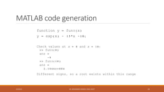
MATLAB provides an easy way to plot symbolic expressions of a single variable, it is
called ezplot. Suppose S is a symbolic expression of x, then
>>ezplot(S, [xmin, xmax])
will plot S between the limits of xmin and xmax.
>> ezplot(S) always uses the range [-2 *pi, 2*pi]
You can use the commands xlabel, ylabel, and title to add x and y labels, etc., in the
usual way. Also use grid on, hold on and hold off, subplots, etc.
4/5/2016 DR. MOHAMMED DANISH/ UNIKL-MICET 8](https://image.slidesharecdn.com/03-chaptermatlabfiniteprecisionarithmatic-200405100512/85/03-Chapter-MATLAB-finite-precision-arithmatic-8-320.jpg)
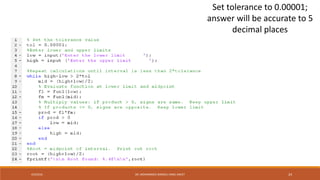


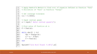
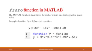
![fzero command in MATLAB
The function fzero has arguments of the name of the function to be evaluated and a guess value:
>> fzero('fun1',10)
ans =
5.6577
Or the name of function to be evaluated and a range of values to be considered:
>> fzero('fun1',[4 10])
ans =
5.6577
4/5/2016 DR. MOHAMMED DANISH/ UNIKL-MICET 44](https://image.slidesharecdn.com/03-chaptermatlabfiniteprecisionarithmatic-200405100512/85/03-Chapter-MATLAB-finite-precision-arithmatic-44-320.jpg)


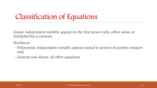
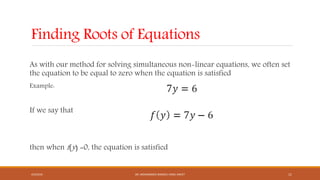
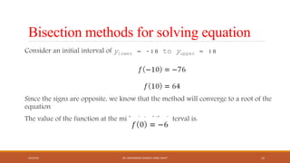
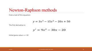
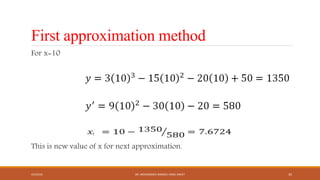
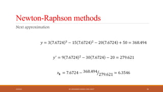
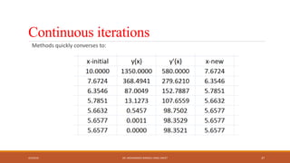
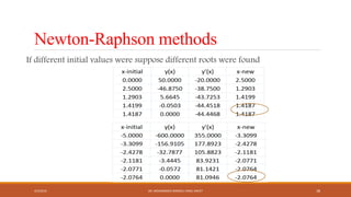
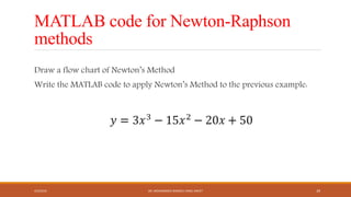
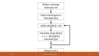
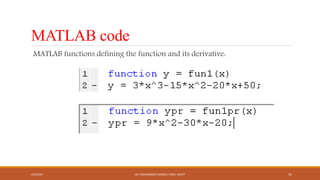
This document discusses numerical methods for finding roots of nonlinear equations. It introduces symbolic calculations in MATLAB using the Symbolic Math Toolbox. Bisection and Newton's methods for finding roots are explained. MATLAB code examples are provided to implement these root-finding algorithms for sample equations. The document also describes using MATLAB's fzero function to numerically find roots.