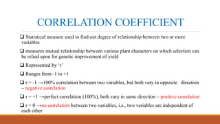
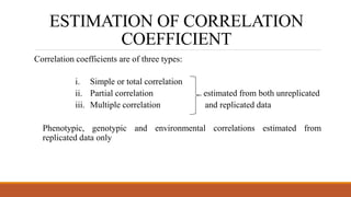
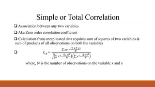
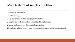
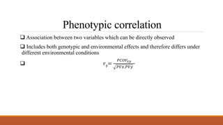
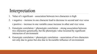
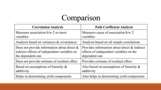
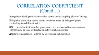
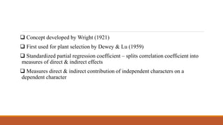
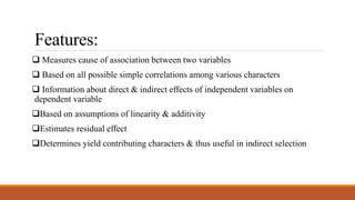
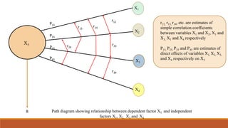
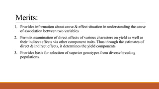
1. Association analysis includes correlation coefficient analysis and path coefficient analysis to study the relationship between two or more variables. 2. Correlation coefficient analysis measures the degree and direction of association between variables on a scale of -1 to 1, where 1 is total positive correlation and -1 is total negative correlation. 3. Path coefficient analysis splits the correlation coefficients into measures of direct and indirect effects to determine the direct and indirect contribution of independent variables to a dependent variable like yield.

1. ASSOCIATION
ANALYSIS

2. Association analysis includes :
1. Correlation coefficient analysis
2. Path coefficient analysis

3. CORRELATION COEFFICIENT
 Statistical measure used to find out degree of relationship between two or more
variables
 measures mutual relationship between various plant characters on which selection can
be relied upon for genetic improvement of yield
 Represented by ‘r’
 Ranges from -1 to +1
 r = -1 →100% correlation between two variables, but both vary in opposite direction
– negative correlation
 r = +1 →perfect correlation (100%), both vary in same direction – positive correlation
 r = 0 →no correlation between two variables, i.e., two variables are independent of
each other

4. CORRELATION COEFFICIENT
(Contd…)
 At genetic level, positive correlation occurs due to coupling phase of linkage
Negative correlation occurs due to repulsion phase of linkage of genes
controlling two different traits
No correlation indicates that genes concerned are located far apart on same
chromosome or they are located on different chromosomes
Nature of correlation – altered by selection & hybridization

5. Properties:
 It is independent of unit of measurement
 Its value lies in between –1 and +1
 It measures the degree and direction of association between two or more
variables

6. ESTIMATION OF CORRELATION
COEFFICIENT
Correlation coefficients are of three types:
i. Simple or total correlation
ii. Partial correlation estimated from both unreplicated
iii. Multiple correlation and replicated data
Phenotypic, genotypic and environmental correlations estimated from
replicated data only

7. Simple or Total Correlation
 Association between any two variables
 Aka Zero order correlation coefficient
 Calculation from unreplicated data requires sum of squares of two variables &
sum of products of all observations on both the variables
 𝑟𝑥𝑦=
𝑥𝑦 −
𝑥. 𝑦
𝑁
𝑥2−
𝑥 2
𝑁
. 𝑦2−
𝑦 2
𝑁
where, N is the number of observations on the variable x and y

8. Main features of simple correlation:
It involves 2 variables
 Denoted as r12
 Ignores effects of other independent variables
 Coefficient of determination cannot be obtained directly
 Value is always lower than multiple correlation
Simple correlation is of 3 types, i.e., phenotypic, genotypic & environmental

9. Phenotypic correlation
 Association between two variables which can be directly observed
 Includes both genotypic and environmental effects and therefore differs under
different environmental conditions
 𝑟p=
𝑃𝐶𝑂𝑉𝑥𝑦
𝑃𝑉𝑥.𝑃𝑉𝑦

10. Genotypic correlation
 Inherent or heritable association between two variables
More stable & is of great importance in breeding – genetic improvement in one
character by selecting other character of a pair that is genetically correlated
 May be either due to pleiotropic action of genes or due to linkage or both
 Association between two traits (whether positive or negative) remains same in parental
population & segregating population – association due to pleiotropy
 Association changes in segregating population – due to linkage between two genes
which has broken in segregating population resulting in recombination between such
genes
 𝑟𝑔 =
𝐺𝐶𝑂𝑉𝑥𝑦
𝐺𝑉𝑥.𝐺𝑉𝑦

11. Environmental correlation
 Entirely due to environmental effects or due to error variance
 Not heritable or stable – less importance in breeding
 𝑟𝑒 =
𝐸𝐶𝑂𝑉𝑥𝑦
𝐸𝑉𝑥. 𝐸𝑉𝑦

12. Interpretation
1. Value of r significant – association between two characters is high
2. r negative – increase in one character lead to decrease in second and vice versa
r positive – increase in one variable cause increase in other and vice versa
3. Genotypic correlation > phenotypic correlation – strong association between
two characters genetically, but the phenotypic value lessened by significant
interaction of environment
4. Genotypic correlation < phenotypic correlation – association of two characters
not only due to genes but also due to favourable influence of environment

13. 5. Environment correlation > Genotypic correlation and phenotypic correlation –
These two characters are showing high association due to favourable influence
of particular environment & this association may change in another locality or
with change in environment
6. Value of r zero or insignificant – two characters are independent

14. Uses:
1. Simple correlations give an idea about co-variation or co-inheritance of two
characters
2. Indicates degree & direction of relationship between two characters
3. Helps in determining the yield contributing characters in plant breeding
Limitations:
1. It assumes a linear relationship between the variables even though it may not be there
2. It is unduly affected by the values of extreme items
3. Calculation is tedious
4. Liable to be misinterpreted as a high degree of correlation does not necessarily mean
very close relationship between variables

15. Partial or Net correlation
 Correlation between two variables (x1 and x2) is worked out by eliminating the
effect of third variable (x3)
Study of relationship between one dependent variable and one independent
variable by keeping other independent variable constant
Estimated from the estimates of simple correlation coefficients

16. Properties:
 It involves 3 or 4 variables
 Denoted as 𝑟12.3 or 𝑟12.34
 Estimated from simple correlations
 Value always lower than multiple correlations
 Does not ignore effects of other variables
 It is of 2 types – first order partial correlation ( r12.3 ) and second order partial
correlation (r12.34)

17. First order partial correlation : Eliminating the effect (keeping constant ) other
characters, one at a time
𝑟12.3=
𝑟12 − 𝑟13.𝑟23
(1−𝑟13
2 )(1−𝑟23
2 )
Where 𝑟12.3 is partial correlation coefficient between variables 1 & 2 by
eliminating the effect of variable 3
◦ 𝑟12.4=
𝑟12 − 𝑟14.𝑟24
(1−𝑟14
2 )(1−𝑟24
2 )

18. Second order partial correlation: Eliminating the effect of other characters,
correlation between two characters at a time is calculated
𝑟12.34=
𝑟12.3 − 𝑟14.3.𝑟24.3
(1−𝑟14.3
2 )(1−𝑟24.3
2 )
𝑟12.34 - second order partial correlation coefficient between variables 1 & 2 by
eliminating effect of variables 3 & 4

19. Interpretation:
1. Value partial correlation coefficient zero – simple correlation between x1 and
x2 is due to effect of another variable x3 but after eliminating effect of x3 , x1
and x2 may be uncorrelated
2. Value of 𝑟12.3 significant –true relationship between x1 and x2

20. Uses:
1. Provides a better insight into true relationship between two variables than is
available from the estimates of simple correlation coefficients between them
2. Does not ignore effects of variables other than which is being studied
3. It is of great importance in plant breeding where yield is the prime objective –
governed by several causal factors
Limitations:
1. Assume that various independent variables are independent of each other –
may not be true in actual practice – interaction among factors may exist
2. Reliability decreases as order goes up
3. Involves lot of calculation work & analysis is not easy

21. Multiple correlation
 Three or more variables studied at a time
 Effect of all independent variables studied on a dependent variable
 Estimate of joint influence of two or more independent variables on a
dependent variable is called multiple correlation coefficient
 Helps in understanding the dependence of one variable x1, on a set of
independent variables x2, x3 etc.
 Measures the joint influence of independent variables x2 and x3 on dependent
variable x1

22. Features:
 Involves several variables
 Denoted by R1.23 , where R is the coefficient of multiple correlation, 1 is the
dependent variable say x1 and 2 and 3 are the independent variables say x2 and x3
 Estimated from simple correlations
 Value always higher than simple and partial correlations
 Non-negative estimate. It can never be negative, hence value lies between 1
and 0

23. Computation:
R1.23=
𝑟12
2 +𝑟13
2 −2𝑟12.𝑟13.𝑟23
1−𝑟23
2
Where R12.3 is the multiple correlation coefficient between the dependent
variable 1 and independent variable 2 and 3

24. Interpretation:
1. Multiple correlation highly significant – dependent variable highly correlated
with independent variables
Coefficient of determination (%) – square of multiple correlation coefficient –
contribution of various components towards dependent variable, say yield

25. Uses:
1. It gives effects of several independent variables on a dependent variable
2. Useful in understanding the changes in the dependent variable
Limitations:
1. Assumes linear relationship between simple or zero order correlation
coefficients
2. Assumes that independent variables affect the independent variable in an
independent manner and have an additive property. If there is interaction
between independent variables their effects cannot be distinct nor can be
additive
3. Calculation is difficult

26. PATH COEFFICIENTANALYSIS

27.  Concept developed by Wright (1921)
 First used for plant selection by Dewey & Lu (1959)
 Standardized partial regression coefficient – splits correlation coefficient into
measures of direct & indirect effects
 Measures direct & indirect contribution of independent characters on a
dependent character

28. Features:
 Measures cause of association between two variables
 Based on all possible simple correlations among various characters
 Information about direct & indirect effects of independent variables on
dependent variable
Based on assumptions of linearity & additivity
Estimates residual effect
Determines yield contributing characters & thus useful in indirect selection

29. Types:
Can be carried out from both unreplicated & replicated data
Unreplicated data – Only simple path worked out
Replicated data – 3 types
Phenotypic path
Genotypic path
Environmental path

30. Phenotypic path
 From phenotypic correlation coefficient
 splits phenotypic correlation coefficients into measures of direct & indirect
effects

31. Genotypic path
 From genotypic correlation coefficient
 splits genotypic correlation coefficients into measures of direct & indirect
effects

32. Environmental path
 From environmental correlation coefficient
 Worked out from all possible environmental correlation coefficients among
various characters included in the study
 Genotypic & phenotypic paths estimated to determine yield contributing
characters – useful for plant breeders in selection of elite genotypes from diverse
genetic population

33. Comparison
Correlation Analysis Path Coefficient Analysis
Measures association b/w 2 or more
variables
Measures cause of association b/w 2
variables
Analysis based on variances & covariances Analysis based on all simple correlations
Does not provide information about direct &
indirect effects of independent variables on
the dependent one
Provides information about direct & indirect
effects of independent variables on the
dependent one
Does not provide estimate of residual effect Provides estimate of residual effect
Based on assumptions of linearity &
additivity
Also based on assumptions of linearity &
additivity
Helps in determining yield components Also helps in determining yield components

34. Computation of Path Coefficients –
Steps:
• Genotypes used should have genetic diversity
• Genotypes may include inbred lines, strains and cultivars
1. Selection
of genotypes
• Selected genotypes evaluated in replicated field experiments
• Observations recorded on various polygenic characters such as
yield and yield contributing factors
2. Evaluation
of material
• Data collected on various polygenic characters subjected to
statistical analysis
• Computation of path coefficients from replicated data involves 3
steps
3. Statistical
Analysis

35. 3. Statistical Analysis
• Estimation of variances & covariances for all characters & their
combinations
• Calculation of all possible simple correlation coefficients among
various characters in study (=
𝑛(𝑛−𝑙)
2
, n is no. of variables)
• Path analysis – consists of calculation of direct effects, indirect effects
and residual effects

36. PATH DIAGRAM
 Line diagram constructed with the help of simple correlation coefficients
among various characters included under study
 Constructed before estimation of direct and indirect effects
 Dependent variable (say yield) is kept on one side and all independent
variables on other side

37. X5
X1
X2
X4
P15
P25
P35
P45
r24
r13
r14
r12
r23
r34
R Path diagram showing relationship between dependent factor X5 and independent
factors X1, X2, X3 and X4
X3
r12, r13, r14, etc. are estimates of
simple correlation coefficients
between variables X1 and X2, X1 and
X3, X1 and X4 respectively
P15, P25, P35 and P45 are estimates of
direct effects of variables X1, X2, X3,
and X4 respectively on X5

38. Uses:
1. Depicts cause & effect situation in a simple manner & makes presentation of
results more attractive
2. Provides visual picture of cause & effect situation
3. Depicts association between various characters
4. Helps in understanding the direct and indirect contribution of various
independent variable towards a dependent variable

39. Direct effects:
 Every component character have a direct effect on yield
 In addition, it also exert indirect effect via other component characters
 Direct effect or contribution of various causal factors is estimated by solving
simultaneous equations, after putting the values of simple correlation coefficients
 Estimates of direct effects, viz., values of P15, P25, P35 and P45 are obtained

40. Indirect effects:
 Effects of an independent character on dependent one via other independent
traits – indirect effects
 Computed by putting values of correlation coefficients and those of direct
effects
Indirect effect of X1 via
X2 = 𝑟12. 𝑃25
X3 = 𝑟13. 𝑃35
X4 = 𝑟14. 𝑃45

41. Similarly, indirect effects of X2 is:
via X1 = 𝑟12. 𝑃15
X3 = 𝑟23. 𝑃35
X4 = 𝑟24. 𝑃45

42. Residual effect:
It measures role of other possible independent variables which were not
included in study on dependent variable
 Estimated with help of direct effects and simple correlation coefficients
1 = 𝑃2
𝑅5 + 𝑃15.𝑟15 + 𝑃25.𝑟25 + 𝑃35.𝑟35 + 𝑃45.𝑟45
where 𝑃2 𝑅5 is the square of residual effect
Therefore, h2 = 𝑃2 𝑅5 = 1 - (𝑃15.𝑟15 + 𝑃25.𝑟25 + 𝑃35.𝑟35 + 𝑃45.𝑟45)

43. Interpretation:
 Direct and indirect effects are rated as follows (Lenka and Mishra, 1973):
0.00 – 0.09 – Negligible
0.10 – 0.19 – Low
0.20 – 0.29 – Moderate
0.30 - 1.00 – High
> 1.00 – Very high

44.  Correlation between yield & a character due to direct effect of a character →
true relationship between them & direct selection for this trait is rewarding for
yield improvement
 Correlation due to indirect effects of character through another component trait
→ indirect selection through such trait in yield improvement
 Direct effect positive and high, but correlation negative – direct selection for
such trait should be practiced to reduce undesirable indirect effect
 Value of residual effect moderate or high – besides the characters that are
studied, there are some other attributes which contribute to yield

45. Merits:
1. Provides information about cause & effect situation in understanding the cause
of association between two variables
2. Permits examination of direct effects of various characters on yield as well as
their indirect effects via other component traits. Thus through the estimates of
direct & indirect effects, it determines the yield components
3. Provides basis for selection of superior genotypes from diverse breeding
populations

46. Demerits:
1. Path analysis is designed to deal with variables having additive effects. Its
application to variables having non-additive effects may lead to wrong results
2. Computation is difficult and inclusion of many variables make the
computation more complicated

47. Thank you