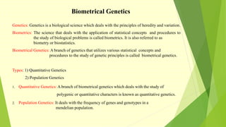
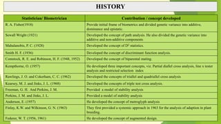
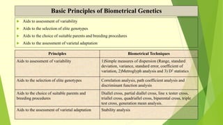
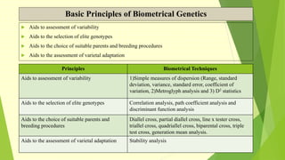
The document discusses biometrical genetics, highlighting its definitions, types, and historical contributions from key statisticians. It elaborates on various analytical techniques used in biometrical genetics, such as quantitative genetics, correlation analysis, path coefficient analysis, and discriminant function analysis, emphasizing their applications in selecting elite genotypes and assessing genetic diversity. Additionally, it compares techniques like metroglyph analysis and d2 statistics, outlining their advantages and disadvantages in genetic studies.

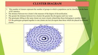


![谷歌留痕技术 [ 𝙩𝙤𝙥 𝟮𝟯𝟯. 𝙘 𝙤𝙢 ]](https://cdn.slidesharecdn.com/ss_thumbnails/top233-260130174328-3833018c-thumbnail.jpg?width=640&height=640&fit=bounds)


