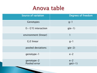
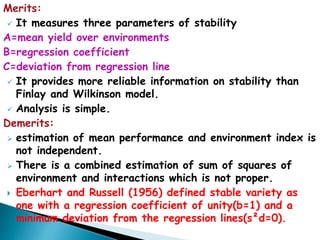
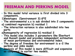
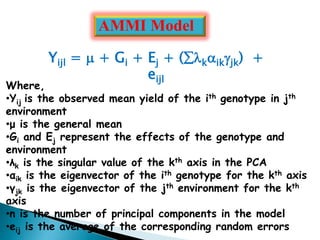
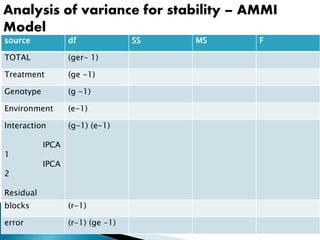
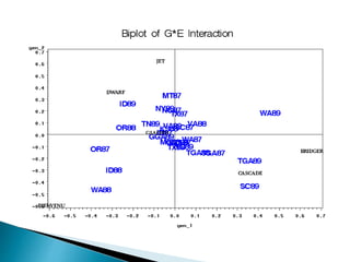
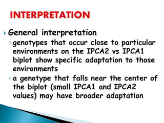
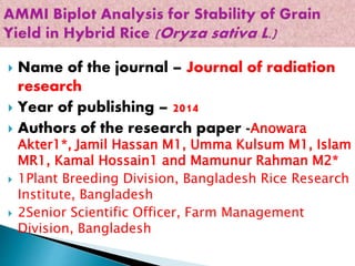
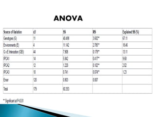
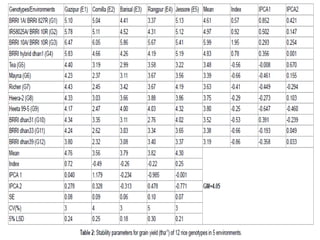
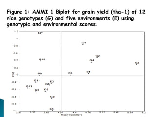
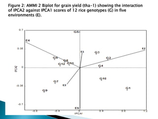
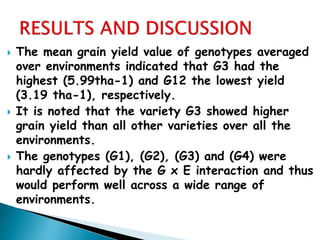
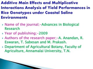
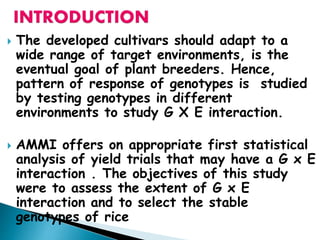
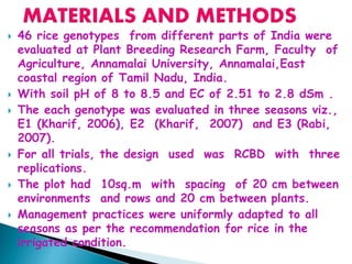
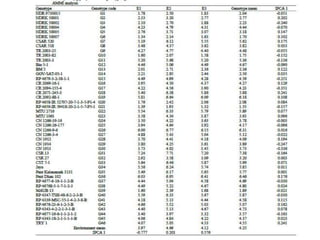
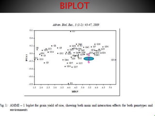
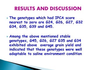
Gene–environment interaction is when two different genotypes respond to environmental variation in different ways. Stability refers to the performance with respective to environmental factors overtime within given location. Selection for stability is not possible until a biometrical model with suitable parameters is available to provide criteria necessary to rank varieties / breeds for stability. Different models of stability are discussed.
It comprises on mating designs used in plant breeding programs. 6 basic mating designs are briefly explained in it with their requirements as well limiting factors...
Power Point is deals with the different aspects of Quantitative genetics in plant breeding it converse Basic Principles of Biometrical Genetics, estimation of Variability, Correlation, Principal Component Analysis, Path analysis, Different Matting design and Stability so on
Mechanism of insect resistance in plants (non preference, antibiosis, tolerance and avoidance) – nature of insect resistance – genetics of insect resistance – horizontal and vertical – genetics of resistance – sources of insect resistance – breeding methods for insect resistance – problems in breeding for insect resistance – achievements.
Stability parameters for comparing varieties (eberhart and russell 1966)Dhanuja Kumar
Phenotype is a result of genotype, environment and GE interaction. GENOTYPE- environment interactions are of major
importance to the plant breeder in developing
improved varieties. The performance of a single variety is not the same in all the environments. To identify a genotype whose performance is stable across environments various models were proposed. One such model was proposed by EBERHART and RUSSELL in 1966. Even after decades, this model is still preferred over others and used till date for stability analysis.
Stability refers to the performance with respective changing environmental factors overtime within given location.
Selection for stability is not possible until a biometrical model with suitable parameters is available to provide criteria necessary to rank varieties / breeds for stability.
The shifted multiplicative model was developed by Cornelius and Seyedsadr in 1992.
SHMM is used to analyze the complete separability, genotypic separability, environmental separability, and inseparability of environment effects and genotypic effects.
Gregorius and Namkoong (1986) defined Separability as the property which is that cultivar effect is separable from environmental effect so that there is no rank.
The shifted multiplicative model (SHMM) is used in an exploratory step-down method for identifying subsets of environments in which genotypic effects are "separable" from environmental effects. Subsets of environments are chosen on the basis of a SHMM analysis of the entire data set. SHMM analyses of the subsets
may indicate a need for further subdivision and/or suggest that a different subdivision at the previous stage should be tried. The process continues until SHMM analysis indicates that a SHMM with only one multiplicative term and its "point of concurrence" outside (left or right) of the cluster of data points adequately fits the data in all subsets.
Advanced biometrical and quantitative genetics akshayAkshay Deshmukh
Additive and Multiplicative Model
Shifted Multiplicative Model
Analysis and Selection of Genotype
Methods and steps to select the best model
Bioplot and mapping genotype
GGEBiplot analysis of genotype × environment interaction in Agropyron interme...Innspub Net
In order to identify genotypes of Agropyron intermedium with high forage yield and stability an experiment was carried out in the Research station of Kermanshah Iran.The 11 accessions were sown in a randomized complete block design with three replications under rainfed and irrigated conditions during 2013-21-014 cropping deasons. Combined analysis of variance indicated high significant differences for location, genotype and G × E interaction (GEI) at 1% level of probability. Mean comparisons over environments introduced G4, G3 and G5 with maximum forage yield over rainfed and irrigated conditions. Minimum forage yield was attributed to genotype G1. GGEbiplot analysis exhibited that the first two principal components (PCA) resulted from GEI and genotype effect justified 99.37% of total variance in the data set. The four environments under investigation fell into two apparent groups: irrigated and rainfed. The presence of close associations among irrigated (E1 and E3) and rainfed (E2 and E4) conditions suggests that the same information about the genotypes could be obtained from fewer test environments, and hence the potential to reduce testing cost.The which-won-where pattern of GGEbiplot introduced genotypes G3 and G4 as stable with high forage yield for rainfed condition, while G5 was stable with high yield for irrigated condition. According to the comparison of the genotypes with the Ideal genotype accessions G4, G3 and G9 were more favorable than all the other genotypes. Get more articles at: http://www.innspub.net/volume-6-number-4-april-2015-jbes/
1. STABILITY OF MALE STERILE LINES - ENVIRONMENTAL INFLUENCE ON STERILITY - EGMS - TYPES AND INFLUENCE ON THEIR EXPRESSION, GENETIC STUDIES.
2. PHOTO SENSITIVE GENETIC MALE STERILITY AND ITS USES IN HETEROSIS BREEDING
3. TEMPERATURE SENSITIVE GENETIC MALE STERILITY AND ITS USES IN HETEROSIS BREEDING
FERTILITY RESTORATION IN MALE STERILE LINES AND RESTORER DIVERSIFICATION PROG...Rachana Bagudam
1. FERTILITY RESTORATION IN MALE STERILE LINES AND RESTORER DIVERSIFICATION PROGRAMMES.
2. CONVERSION OF AGRONOMICALLY IDEAL GENOTYPES INTO MALE STERILES.
3. GENERATING NEW CYTONUCLEAR INTERACTION SYSTEM FOR DIVERSIFICATION OF MALE STERILES.
Gene stacking is a type of gene cloning that refers to the process of combining two or more genes of interest into a single plant. The emerging combined traits from this process are called stacked traits. A genetically engineered crop variety that bears stacked traits is called a biotech stack or simply stack.
Heterotic group “is a group of related or unrelated genotypes from the same or different populations, which display similar combining ability and heterotic response when crossed with genotypes from other genetically distinct germplasm groups.”
Ozone depletion and UV radiations leading to increased ionizing radiations an...Rachana Bagudam
The Earth’s atmosphere is divided into several layers. The lowest region, the troposphere, extends from the Earth’s surface up to about 10 kilometres (km) in altitude. Virtually all human activities occur in the troposphere. Mt. Everest, the tallest mountain on the planet, is only about 9 km high. The next layer, the stratosphere, continues from 10 km to about 50 km. Most commercial airline traffic occurs in the lower part of the stratosphere. For nearly a billion years, ozone molecules in the atmosphere have protected life on Earth from the effects of ultraviolet rays. It is a form of oxygen (O2). We all know that, oxygen we need to live and breathe. Normal oxygen consists of two oxygen atoms. Ozone, however, consists of three oxygen atoms and has the chemical formula O3.
A new era of genomics for plant science research has opened due the complete genome sequencing projects of Arabidopsis thaliana and rice. The sequence information available in public database has highlighted the need to develop genome scale reverse genetic strategies for functional analysis (Till et al., 2003). As most of the phenotypes are obscure, the forward genetics can hardly meet the demand of a high throughput and large-scale survey of gene functions. Targeting Induced Local Lesions in Genome TILLING is a general reverse genetic technique that combines chemical mutagenesis with PCR based screening to identity point mutations in regions of interest (McCallum et al., 2000). This strategy works with a mismatch-specific endonuclease to detect induced or natural DNA polymorphisms in genes of interest. A newly developed general reverse genetic strategy helps to locate an allelic series of induced point mutations in genes of interest. It allows the rapid and inexpensive detection of induced point mutations in populations of physically or chemically mutagenized individuals. To create an induced population with the use of physical/chemical mutagens is the first prerequisite for TILLING approach. Most of the plant species are compatible with this technique due to their self-fertilized nature and the seeds produced by these plants can be stored for long periods of time (Borevitz et al., 2003). The seeds are treated with mutagens and raised to harvest M1 plants, which are consequently, self-fertilized to raise the M2 population. DNA extracted from M2 plants is used in mutational screening (Colbert et al., 2001). To avoid mixing of the same mutation only one M2 plant from each M1 is used for DNA extraction (Till et al., 2007). The M3 seeds produce by selfing the M2 progeny can be well preserved for long term storage. Ethyl methane sulfonate (EMS) has been extensively used as a chemical mutagen in TILLING studies in plants to generate mutant populations, although other mutagens can be effective. EMS produces transitional mutations (G/C, A/T) by alkylating G residues which pairs with T instead of the conservative base pairing with C (Nagy et al., 2003). It is a constructive approach for users to attempt a range of chemical mutagens to assess the lethality and sterility on germinal tissue before creating large mutant populations.
The term balanced tertiary trisomic has three words of which (1) “trisomic” indicates the presence of extra chromosome, (2) “tertiary” indicates that the extra chromosome is a trans-located chromosome, and (3) “balanced” refers to the breeding behaviour of the trisomic.
Ramage defined the BTT as a tertiary trisomic constructed in such a way that the dominant allele of a marker gene, closely linked with the translocation breakpoint of the extra chromosome is carried on the extra chromosome, and the recessive allele is carried on the two normal chromosomes that constitute the diploid complement. The dominant marker gene may be located on the centromere segment or the trans-located segment of the extra chromosome.
The concept of gene for gene hypothesis was first developed by Flor in 1956 based on his studies of host pathogen interaction in flax, for rust caused by Melampsora lini. The gene for gene hypothesis states that for each gene controlling resistance in the host, there is corresponding gene controlling pathogenicity in the pathogen. The resistance of host is governed by dominant genes and virulence of pathogen by recessive genes. The genotype of host and pathogen determine the disease reaction. When genes in host and pathogen match for all loci, then only the host will show susceptible reaction. If some gene loci remain unmatched, the host will show resistant reaction. Now gene – for –gene relationship has been reported in several other crops like potato, sorghum, wheat, etc. The gene for gene hypothesis is also known as “Flor Hypothesis.”
Plants are continually exposed to harsh environmental conditions which is life- threatening for their survival. Drought is one of the major environmental constraints that highly affect plant growth and productivity worldwide. Osmotic stress due to limited availability of water during drought lead to the inhibition of photosynthesis which ultimately affect plant growth, yield and productivity. As sessile in nature, plants cannot escape from such adverse situations. Hence, to cope up with these adverse situations, plants have developed a complex array of adaptive strategies including intricate regulation of cellular, physiological, biochemical and metabolic processes to avoid or tolerate cellular dehydration. Under limited water availability, stomata plays an essential role to check water loss due to transpiration. In addition, upon perception of stress signal, a wide range of signaling cascade has been activated which ultimately initiates the expression of stress-responsive genes in a timely and coordinated manner. Abscisic acid (ABA), the universal stress hormone, highly accumulated under stress condition, also plays an important role in stress adaptation including stomatal closure and expression of stress-responsive genes. In recent times, whole genome sequencing analysis of different plants reveals that a large family of genes is expressed under different types of abiotic stresses that are involved in defense-related pathways. These genes can be grouped into three categories, genes involving recognition of osmotic stress, signal perception, and transduction and production of stress-adaptive components for physiological responses.
The nanotechnology aided applications have the potential to change agricultural production by allowing better management and conservation of inputs of plant and animal production. Several nanotechnology applications for agricultural production for developing countries within next 10 years has been predicted (Salamanca–Buentella et al., 2005).
Nanoparticles helps in Controlling the Plant Diseases, application of agricultural fertilizers, pesticides, antibiotics, and nutrients is typically by spray or drench application to soil or plants, or through feed or injection systems to animals. In this context, nanotechnologies offer a great opportunity to develop new products against pests (Caraglia et al., 2011). Nanoscale devices are envisioned that would have the capability to detect and treat an infection, nutrient deficiency, or other health problem, long before symptoms were evident at the macro-scale. The overall goal of this Nanoparticles is to reduce the number of unnecessary problems in agriculture (Thomas et al., 2011). In the management aspects, efforts are made to increase the efficiency of applied fertilizer with the help of nano clays and zeolites and restoration of soil fertility by releasing fixed nutrients (Dongling Qiao, et al., 2016). Nanoherbicides are being developed to address the problems in perennial weed management and exhausting weed seed bank. Bioanalytical Nanosensors are utilized to detect and quantify minute amounts of contaminants like viruses bacteria, toxins bio-hazardous substances etc. in agriculture and food systems (Tothill EI, 2011).
In this way, nanotechnology can be used as an innovative tool for delivering agrochemicals safely. More research should be done on the potential adverse effects of nanomaterials on human health, crops and the environmental safety. It is a challenge to Government and private sector as they have to ensure the acceptance of Nano foods. For it to flourish, continuous funding and understanding on the part of policy makers and science administrators, along with reasonable expectations, would be crucial for this promising field.
Cancer cell metabolism: special Reference to Lactate PathwayAADYARAJPANDEY1
Normal Cell Metabolism:
Cellular respiration describes the series of steps that cells use to break down sugar and other chemicals to get the energy we need to function.
Energy is stored in the bonds of glucose and when glucose is broken down, much of that energy is released.
Cell utilize energy in the form of ATP.
The first step of respiration is called glycolysis. In a series of steps, glycolysis breaks glucose into two smaller molecules - a chemical called pyruvate. A small amount of ATP is formed during this process.
Most healthy cells continue the breakdown in a second process, called the Kreb's cycle. The Kreb's cycle allows cells to “burn” the pyruvates made in glycolysis to get more ATP.
The last step in the breakdown of glucose is called oxidative phosphorylation (Ox-Phos).
It takes place in specialized cell structures called mitochondria. This process produces a large amount of ATP. Importantly, cells need oxygen to complete oxidative phosphorylation.
If a cell completes only glycolysis, only 2 molecules of ATP are made per glucose. However, if the cell completes the entire respiration process (glycolysis - Kreb's - oxidative phosphorylation), about 36 molecules of ATP are created, giving it much more energy to use.
IN CANCER CELL:
Unlike healthy cells that "burn" the entire molecule of sugar to capture a large amount of energy as ATP, cancer cells are wasteful.
Cancer cells only partially break down sugar molecules. They overuse the first step of respiration, glycolysis. They frequently do not complete the second step, oxidative phosphorylation.
This results in only 2 molecules of ATP per each glucose molecule instead of the 36 or so ATPs healthy cells gain. As a result, cancer cells need to use a lot more sugar molecules to get enough energy to survive.
introduction to WARBERG PHENOMENA:
WARBURG EFFECT Usually, cancer cells are highly glycolytic (glucose addiction) and take up more glucose than do normal cells from outside.
Otto Heinrich Warburg (; 8 October 1883 – 1 August 1970) In 1931 was awarded the Nobel Prize in Physiology for his "discovery of the nature and mode of action of the respiratory enzyme.
WARNBURG EFFECT : cancer cells under aerobic (well-oxygenated) conditions to metabolize glucose to lactate (aerobic glycolysis) is known as the Warburg effect. Warburg made the observation that tumor slices consume glucose and secrete lactate at a higher rate than normal tissues.
This pdf is about the Schizophrenia.
For more details visit on YouTube; @SELF-EXPLANATORY;
https://www.youtube.com/channel/UCAiarMZDNhe1A3Rnpr_WkzA/videos
Thanks...!
Observation of Io’s Resurfacing via Plume Deposition Using Ground-based Adapt...Sérgio Sacani
Since volcanic activity was first discovered on Io from Voyager images in 1979, changes
on Io’s surface have been monitored from both spacecraft and ground-based telescopes.
Here, we present the highest spatial resolution images of Io ever obtained from a groundbased telescope. These images, acquired by the SHARK-VIS instrument on the Large
Binocular Telescope, show evidence of a major resurfacing event on Io’s trailing hemisphere. When compared to the most recent spacecraft images, the SHARK-VIS images
show that a plume deposit from a powerful eruption at Pillan Patera has covered part
of the long-lived Pele plume deposit. Although this type of resurfacing event may be common on Io, few have been detected due to the rarity of spacecraft visits and the previously low spatial resolution available from Earth-based telescopes. The SHARK-VIS instrument ushers in a new era of high resolution imaging of Io’s surface using adaptive
optics at visible wavelengths.
(May 29th, 2024) Advancements in Intravital Microscopy- Insights for Preclini...Scintica Instrumentation
Intravital microscopy (IVM) is a powerful tool utilized to study cellular behavior over time and space in vivo. Much of our understanding of cell biology has been accomplished using various in vitro and ex vivo methods; however, these studies do not necessarily reflect the natural dynamics of biological processes. Unlike traditional cell culture or fixed tissue imaging, IVM allows for the ultra-fast high-resolution imaging of cellular processes over time and space and were studied in its natural environment. Real-time visualization of biological processes in the context of an intact organism helps maintain physiological relevance and provide insights into the progression of disease, response to treatments or developmental processes.
In this webinar we give an overview of advanced applications of the IVM system in preclinical research. IVIM technology is a provider of all-in-one intravital microscopy systems and solutions optimized for in vivo imaging of live animal models at sub-micron resolution. The system’s unique features and user-friendly software enables researchers to probe fast dynamic biological processes such as immune cell tracking, cell-cell interaction as well as vascularization and tumor metastasis with exceptional detail. This webinar will also give an overview of IVM being utilized in drug development, offering a view into the intricate interaction between drugs/nanoparticles and tissues in vivo and allows for the evaluation of therapeutic intervention in a variety of tissues and organs. This interdisciplinary collaboration continues to drive the advancements of novel therapeutic strategies.
Richard's entangled aventures in wonderlandRichard Gill
Since the loophole-free Bell experiments of 2020 and the Nobel prizes in physics of 2022, critics of Bell's work have retreated to the fortress of super-determinism. Now, super-determinism is a derogatory word - it just means "determinism". Palmer, Hance and Hossenfelder argue that quantum mechanics and determinism are not incompatible, using a sophisticated mathematical construction based on a subtle thinning of allowed states and measurements in quantum mechanics, such that what is left appears to make Bell's argument fail, without altering the empirical predictions of quantum mechanics. I think however that it is a smoke screen, and the slogan "lost in math" comes to my mind. I will discuss some other recent disproofs of Bell's theorem using the language of causality based on causal graphs. Causal thinking is also central to law and justice. I will mention surprising connections to my work on serial killer nurse cases, in particular the Dutch case of Lucia de Berk and the current UK case of Lucy Letby.
2. The interaction between the genotype
and environment that produces the
phenotype is called as Genotype x
Environmental Interaction.
P = G + E + GE
Genotypes respond differently across
a range of environments i.e., the
relative performance of varieties
depends on the environment.
3. Environmental variable can be divided into 2
groups (Allard and Bradshaw , 1964)
1.Predictable environment factor
2.Unpredictable factor
Predictable factors include permanent features
of environment which are under human control
such as soil type, planting date, row spacing,
rows of new trend application.
Unpredictable factors are those which
fluctuate inconsistently like rainfall,
temperature, relative humidity not under
control are called unpredictable environment
conditions.
4. The environment refers to the external
conditions that affect expression of
genes of an individual genotype.
Environment can be classified into two
groups ( Comstock and Moll , 1963)
a) macro environment
b) micro environment
5. Refers to the environment with variables having
large and easily recognisable effect.
Main features:
1. The environment affects are easily
detectable such as fertilizer doses, planting
dates, spacing, irrigation schedules.
2. Macro environment is controlled by
Predictable factors such as soil type, planting
dates and close spacing.
3. It is under human control
6. The environment of a single organism
/genotype as opposed to that of another
growing at the same time in almost the same
place is referred to as micro environment.
Main features:
1.The environment effects are not easily
recognizable such as differences in humidity
, temperature, etc.. at the same place.
2.Micro environment is governed by
unpredictable factors like rain fall,
temperature, relative humidity which
fluctuate inconsistently.
3.It is not under human control.
7. It refers to those changes in structure or
function of an individual/population which lead to
better survival in a given environment is known
as adaptation.
Main features:
₭ Adaptation favours those characters which are
advantageous for survival and through which an
individual acquires adaptive value or fitness.
₭ In the process of adaptation survival is the main
concern.
₭ Natural selection plays an important role in the
process of adaptation.
ADAPTATION
8. TYPES OF ADAPTATION
There are four types of adaptation
1.Specific genotypic adaptation
2.General genotypic adaptation
3.Specific population adaptation
4.General population adaptation
Factors affecting adaptability:
Heterogeneity.
Heterozygosity.
Genetic polymorphism.
Mode of pollination.
9. Stability refers to the performance with
respective changing environmental factors
overtime within given location.
selection for stability is not possible until
a biometrical model with suitable
parameters is available to provide criteria
necessary to rank varieties / breeds for
stability.
Low magnitude of G.E interaction involves
the consistent performance of a population
over variable environments.
10. It consists of following steps:
Location / environment wise analysis of
variance.
pooled analysis of variance for all the
locations/ environments.
If G.E interaction is found significant
,stability analysis can be carried out using
one of the four methods:
1.Finlay and Wilkinson model (1963)
2.Eberhat and Russell model(1966)
3.Perkins and Jinks model(1968)
4.Freeman and Perkins model (1971)
11. Used two parameters
1)Mean performance over environments.
2)Regression performance in different
environments.
The following inferences can be drawn:
1)The regression coefficient of unity indicates
average stability
2)If the regression coefficient is >1,it means
below average stability
3) If the regression coefficient is <1,it means
above average stability.
4) Regression coefficient of 0 would express
absolute stability.
12. MERITS
Analysis of this model is simple.
2 parameters- mean yield over locations and
regression coefficient are used to asses the
phenotypic stability.
DEMERITS
The deviations from the regression line are not
estimated which are important for the stability
analysis.
Greater emphasis is given on mean performance
over environments than regression coefficients.
13. It is the most popular and useful model.
In 1966 both made further improvement in stability
analysis by partitioning the G.E interaction of each
variety into 2 parts. one is slope of the regression line ,
second is deviation from regression line.
In this model total variance is first divided into 2
components:
-genotypes
-environment plus interaction (E+G*E)
The second component is further divided in to 3
components.
I. Environment linear
II. G.E linear
III. Pooled deviations
Sum of squares due to pooled deviations are further
divided into sum of squares due to individual genotype.
14. This model consists of three parameters
a) mean yield over locations
b)regression coefficient =bi
C)Deviation from regression =s²di
Analysis of stability parameters is simple as
compared to other models of stability analysis.
The degree of freedom for environment is 1.
It requires less area hence less expensive when
compared to other models.
It does not provide independent estimation for
mean performance and environmental index
15. Source of variation Degrees of freedom
Genotypes g-1
E+ G*E interaction g(e-1)
environment (linear) 1
G.E linear g-1
pooled deviations g(e-2)
genotype-1 e-2
genotype-2
Pooled error
e-2
ge(r-1)
16. Merits:
It measures three parameters of stability
A=mean yield over environments
B=regression coefficient
C=deviation from regression line
It provides more reliable information on stability than
Finlay and Wilkinson model.
Analysis is simple.
Demerits:
estimation of mean performance and environment index is
not independent.
There is a combined estimation of sum of squares of
environment and interactions which is not proper.
Eberhart and Russell (1956) defined stable variety as
one with a regression coefficient of unity(b=1) and a
minimum deviation from the regression lines(s²d=0).
17. In this model total variance is first divided into 3
components.
1)genotypes
2)environments
3)genotypes x environment
G-E variance is sub divided into
a) heterogeneity due to regression
b) sum of square due to remainder
This model is less expensive than Freeman and Perkins.
It requires less area for experimentation.
The degree of freedom for environment is e-2.
Analysis is more difficult than Eberhart and Russell
model.
It does not provide independent estimation of mean
performance and environmental index.
18. Source of variation Degrees of freedom
Genotypes g-1
Environment e-1
Genotype x environment (g-1)(e-1)
Heterogeneity among regressions g-1
Remainder (g-1)(e-2)
Error ge(r-1)
19. In this model total variance is first divided into 3
components.
1)Genotypes 2)environment 3) G*E
The environmental s.s is sub divided into 2 components
a) combined regression b) residual 1
The interaction variance is also subdivided into two
parts
a)homogeneity of regression b) residual 2
This model also includes 3 parameters like Eberhart
and Russell model and provides independent estimation
of mean performance and environmental index.
The degree of freedom for environment is e-2 like
perkins and jinks model.
Analysis of this model is more difficult and expensive
as compared to earlier two models.
20. Source of variation Degrees of freedom
Genotypes g-1
Environment e-1
Combined regression 1
residual (1) e-2
Interaction(GxE) (g-1)(e-2)
Heterogeneity of regressions g-1
residual (2)
error
(g-1)(e-2)
ge(r-1)
21. AMMI is a combination of ANOVA for the main
effects of the genotypes and the environment
together with principal components analysis of
the genotype-environment interaction.
Method for analyzing GEI to identify patterns of
interaction and reduce background noise.
May provide more reliable estimates of genotype
performance than the mean across sites.
Biplots help to visualize relationships among
genotypes and environments; show both main and
interaction effects.
22. Yijl = + Gi + Ej + (kikjk) +
eijl
Where,
•Yij is the observed mean yield of the ith genotype in jth
environment
•μ is the general mean
•Gi and Ej represent the effects of the genotype and
environment
•λk is the singular value of the kth axis in the PCA
•αik is the eigenvector of the ith genotype for the kth axis
•γjk is the eigenvector of the jth environment for the kth
axis
•n is the number of principal components in the model
•eij is the average of the corresponding random errors
AMMI Model
23. source df SS MS F
TOTAL (ger- 1)
Treatment (ge -1)
Genotype (g -1)
Environment (e-1)
Interaction
IPCA
1
IPCA
2
Residual
(g-1) (e-1)
blocks (r-1)
error (r-1) (ge -1)
Analysis of variance for stability – AMMI
Model
24. PRINCIPAL COMPONENTS
usually the first principal component (CP1)
represents responses of the genotypes
that are proportional to the
environments, which are associated with
the GxE interaction without change of the
range.
The second principal component (CP2)
provides information about cultivation
locations that are not proportional to the
environments, indicating that those are
responsible of the GxE crossover
interaction.
25. Biplot allows the observation in the same graph
of the genotypes (points) and the environments
(vectors), and (2) the exploration of patterns
attributable to the effects of GxE interaction.
In the biplot, the angles between the vectors
that represent genotypes and environments show
the interaction, and the distances from the
origin indicate the degree of interaction that
the genotypes show throughout the environments
or vice versa.
Graphical representation of numerical results
often allows a straight forward interpretation
of GEI.
BIPLOTS
26.
27. General interpretation
◦ genotypes that occur close to particular
environments on the IPCA2 vs IPCA1
biplot show specific adaptation to those
environments
◦ a genotype that falls near the center of
the biplot (small IPCA1 and IPCA2
values) may have broader adaptation
28. How many IPCAs (interaction principal component
axes) are needed to adequately explain patterns
in the data?
◦ Rule of thumb - discard higher order IPCAs
until total SS due to discarded IPCA's ~ SSE.
◦ Usually need only the first 2 PC axes to
adequately explain the data (IPCA1 and
IPCA2). This model is referred to as AMMI2.
Approach is most useful when G x location
effects are more important than G x year
effects
29. Name of the journal – Journal of radiation
research
Year of publishing – 2014
Authors of the research paper -Anowara
Akter1*, Jamil Hassan M1, Umma Kulsum M1, Islam
MR1, Kamal Hossain1 and Mamunur Rahman M2*
1Plant Breeding Division, Bangladesh Rice Research
Institute, Bangladesh
2Senior Scientific Officer, Farm Management
Division, Bangladesh
30. Genotype x environment interaction and stability
performance were investigated on grain yield
with 12 rice genotypes in five environments.
The ANOVA for grain yield revealed highly
significant (P<0.01) for genotypes, environments
and their interactions.
The significant interaction indicated that the
genotypes respond differently across the
different environments.
31. The AMMI model is a hybrid model involving both
additive and multiplicative components of two way
data structure which enabled a breeder to get
precise prediction on genotypic potentiality and
environmental influences on it.
AMMI uses ordinary ANOVA to analyze the main
effects (additive part) and PCA to analyze the non
additive residual left over by the ANOVA .
The main objectives of the present study are to
identify more high yielding stable promising
hybrids and to determine the areas where rice
hybrids would be adapted by AMMI model.
32. The experiments were conducted at five districts
namely Gazipur(E1), Comilla (E2), Barisal (E3),
Rangpur (E4) and Jessore (E5) representing five
different agro-ecological zones (AEZ) of
Bangladesh.
Twelve genotypes consisting of 3 advanced lines
(BRRI 1A/ BRRI 827R(G1), IR58025A/ BRRI 10R
(G2) and BRRI 10A/ BRRI 10R (G3)), 6released
hybrids (BRRI hybrid dhan1(G4), Tea (G5), Mayna
(G6),Richer (G7), Heera-2 (G8) and Heeta 99-5
(G9)), and 3 inbred check varieties (BRRI dhan31
(G10), BRRI dhan33 (G11) and BRRI dhan39(G12))
were used as experimental materials.
33. The experiments were carried out in a randomized
complete block design (RCBD), with 3 replications.
21 days old seedlings were transplanted in 20
square meter plot using single seedling per hill at
a spacing of 20 cm×15cm.
Fertilizers were applied @ 150:100:70:60:10
kg/ha Urea, TSP,MP, gypsum and ZnSO4,
respectively.
Standard agronomic practices were followed and
plant protection measures were taken as required.
The grain yield data for 12 genotypes in 5
environments were subjected to AMMI analysis of
variance using statistical analysis package
software Cropstat version 6.1
36. Figure 1: AMMI 1 Biplot for grain yield (tha-1) of 12
rice genotypes (G) and five environments (E) using
genotypic and environmental scores.
37. Figure 2: AMMI 2 Biplot for grain yield (tha-1) showing the interaction
of IPCA2 against IPCA1 scores of 12 rice genotypes (G) in five
environments (E).
38. The mean grain yield value of genotypes averaged
over environments indicated that G3 had the
highest (5.99tha-1) and G12 the lowest yield
(3.19 tha-1), respectively.
It is noted that the variety G3 showed higher
grain yield than all other varieties over all the
environments.
The genotypes (G1), (G2), (G3) and (G4) were
hardly affected by the G x E interaction and thus
would perform well across a wide range of
environments.
39. Name of the journal;-Advances in Biological
Research
Year of publishing;-2009
Authors of the research paper;-A. Anandan, R.
Eswaran, T. Sabesan and M. Prakash.
Department of Agricultural Botany, Faculty of
Agriculture, Annamalai University, T.N.
40. ABSTRACT:
The objective of the present investigation was
to analyse the pattern of Genotype x
Environment (G x E) interaction for grain yield
of 46 genotypes by Additive Main effects and
Multiplicative Interaction (AMMI) model using
the data generated from three saline stress
environments of east coastal region of Tamil
Nadu, India.
The results showed highly significant genotypic
and G x E interaction.
The G x E interaction influenced the relative
ranking of the genotypes across saline stress
environment condition.
41. The developed cultivars should adapt to a
wide range of target environments, is the
eventual goal of plant breeders. Hence,
pattern of response of genotypes is studied
by testing genotypes in different
environments to study G X E interaction.
AMMI offers on appropriate first statistical
analysis of yield trials that may have a G x E
interaction . The objectives of this study
were to assess the extent of G x E
interaction and to select the stable
genotypes of rice
42. 46 rice genotypes from different parts of India were
evaluated at Plant Breeding Research Farm, Faculty of
Agriculture, Annamalai University, Annamalai,East
coastal region of Tamil Nadu, India.
With soil pH of 8 to 8.5 and EC of 2.51 to 2.8 dSm .
The each genotype was evaluated in three seasons viz.,
E1 (Kharif, 2006), E2 (Kharif, 2007) and E3 (Rabi,
2007).
For all trials, the design used was RCBD with three
replications.
The plot had 10sq.m with spacing of 20 cm between
environments and rows and 20 cm between plants.
Management practices were uniformly adapted to all
seasons as per the recommendation for rice in the
irrigated condition.
46. The genotypes which had IPCA score
nearest to zero are G24, G26, G27, G32
G34, G35, G39 and G45.
Among the above mentioned stable
genotypes, G45, G26, G27 G35 and G34
exhibited above average grain yield and
indicated that these genotypes were well
adaptable to saline environment condition