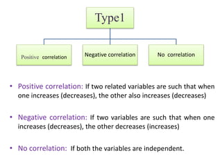
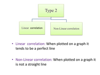
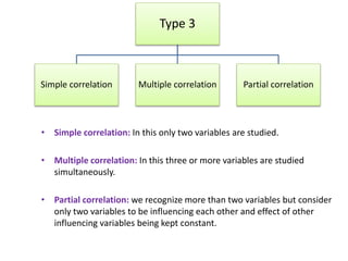
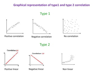
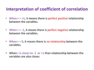
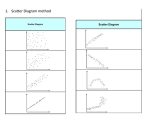
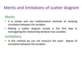
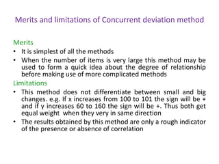
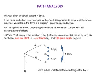
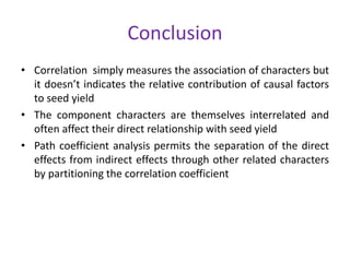
This document discusses correlation coefficient and path coefficient analysis. It defines correlation as a statistical method to analyze the relationship between two or more variables. Correlation determines the degree of relationship but not causation. The document then discusses different types of correlation including positive, negative, linear, non-linear, simple, multiple and partial correlation. It also discusses methods to measure correlation including scatter diagrams, Karl Pearson's coefficient, Spearman's coefficient and concurrent deviation method. Finally, it explains path analysis which can be used to partition correlations into direct and indirect effects when studying causal relationships between variables.

1. Correlation coefficient and path coefficient analysis
By
RajeshRanjanandAmitKumarGaur
PAU,Ludhiana ,Punjab

2. What is correlation?
Correlation is a statistical device which help in analyzing the
covariation of two or more variables.
It helps us in determining the degree of relationship between
two or more variables.
But it does not tell us about cause and effect relationship.
Correlation analysis consist of two simple steps:
Determining whether a relationship exists and, if it
does, measuring it.
Testing whether it is significant.

3. Why we study correlation?
• To find the nature of relationship between two or more
variables.
• To estimate the value of one variable if the value of another
is given.
• To reduce the range of uncertainty. The prediction based on
correlation analysis is likely to be more valuable and near to
reality.

4. What are the reasons for correlation between variables?
• It may be due to pure chance, especially in a small variables in
a sample. But in the universe there may not be any
relationship between the variables.
• Both the correlated variables may be influenced by one or
more other variables e.g. a high degree of correlation
between the yield/acre of rice and tea may be due to the fact
that both are related to amount of rainfall.
• Both the variables may be mutually influencing each other so
that neither can be designated as cause and effects e.g. price
and demand.

5. Different types of correlations
There are three ways to classify the correlation
1. Type 1
• Positive correlation
• Negative correlation
• No correlation
2. Type 2
• Linear correlation
• Non linear correlation
3. Type 3
• Simple correlation
• Multiple correlation
• Partial correlation

6. Type1
Positive correlation Negative correlation No correlation
• Positive correlation: If two related variables are such that when
one increases (decreases), the other also increases (decreases)
• Negative correlation: If two variables are such that when one
increases (decreases), the other decreases (increases)
• No correlation: If both the variables are independent.

7. • Linear correlation: When plotted on a graph it
tends to be a perfect line
• Non-Linear correlation: When plotted on a graph it
is not a straight line
Type 2
Linear correlation Non-Linear correlation

8. • Simple correlation: In this only two variables are studied.
• Multiple correlation: In this three or more variables are studied
simultaneously.
• Partial correlation: we recognize more than two variables but consider
only two variables to be influencing each other and effect of other
influencing variables being kept constant.
Type 3
Simple correlation Multiple correlation Partial correlation

9. Positive correlation Negative correlation No correlation
Positive linear Negative linear Non linear
Graphical representation of type1 and type 2 correlation
Type 1
Type 2

10. Interpretation of coefficient of correlation
• When r = +1, it means there is perfect positive relationship
between the variables.
• When r = -1, it means there is perfect negative relationship
between the variables.
• When r = 0, it means there is no relationship between the
variables.
• When r is closer to -1 or +1 than relationship between the
variables are also closer.

11. Properties of coefficient of correlation
• The coefficient of correlation lies between -1 to +1.
• The coefficient of correlation is independent of change of
scale and origin of the variable x & y.
• The degree of relationship between the two variables is
symmetric 𝑟𝑥𝑦= 𝑟𝑦𝑥.

12. Coefficient of determination
It is a useful way of interpreting the value of coefficient of
correlation between two variables
Coefficient of determination (𝐫𝟐) =
For example If the value of r = 0.9 than r2
=0.81 it means 81% of
the variation in the dependent variable has been explained by
the independent variable
Explained variance
Total variance

13. Properties of coefficient of determination
• Its range lies between 0 to 1
• Represented by r2
• The coefficient of determination is a measure of how well the regression line
represents the data
• If the regression line passes exactly through every point on the scatter plot, it
would be able to explain all of the variation
• The further the line is away from the points, the less it is able to explain

14. Methods of studying correlation
1. Scatter diagram method
2. Karl’s Pearson coefficient of correlation
3. Spearman’s coefficient of correlation
4. Concurrent deviation method

15. 1. Scatter Diagram method
Scatter Diagram Scatter Diagram

16. Merits and limitations of scatter diagram
Merits
• It is simple and non mathematical methods of studying
correlation between the variables
• Making a scatter diagram usually is the first step in
investigating the relationship between two variables
Limitations
• In this method we can not measure the exact degree of
correlation between the variables

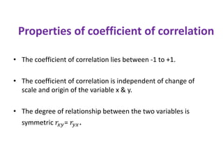
17. Karl Pearson’s Correlation Coefficient
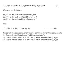
Karl Pearson (1857-1936) British mathematician and statistician
r = 1/N[ (X – X) (Y – Y)]
1/N(X – X)2 1/N(Y – Y)2
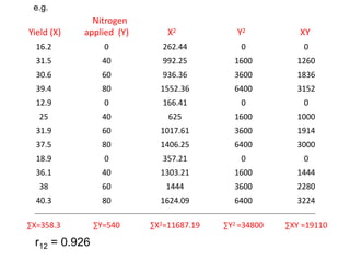
r = N(XY) – (X) (Y)
[N X2 – (X)2] [NY2 – (Y)2]
r = Covariance ( X, Y)
SD (X) . SD (Y)
An alternative computational equation is given below.
The extent to which two variables vary together is called covariance
and its measurement is the correlation coefficient
Where N= No. of Pairs
or

18. Yield (X)
Nitrogen
applied (Y) X2 Y2 XY
16.2 0 262.44 0 0
31.5 40 992.25 1600 1260
30.6 60 936.36 3600 1836
39.4 80 1552.36 6400 3152
12.9 0 166.41 0 0
25 40 625 1600 1000
31.9 60 1017.61 3600 1914
37.5 80 1406.25 6400 3000
18.9 0 357.21 0 0
36.1 40 1303.21 1600 1444
38 60 1444 3600 2280
40.3 80 1624.09 6400 3224
∑X=358.3 ∑Y=540 ∑X2=11687.19 ∑Y2 =34800 ∑XY =19110
r12 = 0.926
e.g.

19. Test for Significance of Observed Correlation Coefficient
Null Hypothesis Ho: ρ = 0
Alternative Hypothesis H1: ρ ≠ 0 ( Two tailed test)
Test Statistics
t = r √ n-2 ~ tα/2, n-2 d.f
√ 1- r2
Where r is the sample correlation coefficient.
If t cal ≤ tα/2, n-2 d.f we don’t enough evidence to reject Ho
Example : Calculated value of r is 7.75 at 10 d.f at 1% level of significance
( t = 3.169)
Conclusion : No- Significant Correlation exists between yield and Nitrogen applied

20. Merits and limitations of Karl Pearson’s
Correlation Coefficient
Merits
• It is most popular method used for measuring the degree
of relationship.
• It helps us to find the exact degree of correlation
Limitations
• The correlation coefficient always assumes linear
relationship regardless of the fact whether assumption is
correct or not
• Takes more time to computes correlation coefficient

21. Spearman’s Coefficient of correlation
• A method to determine correlation when the data is not available in numerical
form and as an alternative, the method of rank correlation is used.
• Thus when the values of the two variables are converted to their ranks, and
there from the correlation is obtained, the correlations known as rank
correlation.
This method was developed by British psychologist Charles Edward Spearman in 1904

22. 𝑟𝑠= 1- 6 { 𝐷2 + 1
12
(𝑚3- m) + 1
12
(𝑚3
- m) + ………}
𝑁3-N
Where, m= number of times common ranks are repeated
x Rank y Rank
Var 1 3 Var 1 1 4
Var 2 7 Var 2 6 1
Var 3 6 Var 3 4 4
Var 4 4 Var 4 2 4
Var 5 5 Var 5 3 4
Var 6 1 Var 6 7 36
Var 7 2 Var 7 5 9
62
(𝑅𝑥−𝑅𝑦) 2
𝐷2
2

23. By using the formula
𝑟𝑠 = 1- 6 x 62 / 73
-7
= 1-1.107
Hence, 𝑟𝑠 = - 0.107

24. Merits and limitations of Spearman’s coefficient of correlation
Merits
• This method is simpler to understand and easier to apply
as compared to the Karl pearson’s method
• This method can be used with great advantage where the
data are of a qualitative in nature
Limitations
• This method should not be applied where N exceeds 30
because the calculations become tedious and require a lot of
time

25. Concurrent deviation method
Steps involved in this methods are
1. Find out the direction of change of x variable as compared with
the first value whether, second value is increasing or decreasing or
constant, and denote this column by 𝐷𝑥
2. If it is increasing put a (+) sign and if decreasing (–) sign and if
constant than put 0
3. Similarly we can do it for y variable and denote this column by 𝐷𝑦
4. Multiply 𝐷𝑥 with 𝐷𝑦 and find value of C, i.e. is number of (+) sign

26. ± 2𝐶 − 𝑛/𝑛
𝑟𝑐 = ±
x 𝐷𝑥 y 𝐷𝑦 𝐷𝑥 x 𝐷𝑦
60 65
55 - 40 - +
50 - 35 - +
56 + 75 + +
30 - 63 - +
70 + 80 + +
40 - 35 - +
35 - 20 - +
80 + 80 + +
80 0 60 - 0
75 - 60 0 0
C= 8
𝑟𝑐 = ± ± 2𝐶 − 𝑛/𝑛 = 6/10 = 0.774

27. Merits and limitations of Concurrent deviation method
Merits
• It is simplest of all the methods
• When the number of items is very large this method may be
used to form a quick idea about the degree of relationship
before making use of more complicated methods
Limitations
• This method does not differentiate between small and big
changes. e.g. If x increases from 100 to 101 the sign will be +
and if y increases 60 to 160 the sign will be +. Thus both get
equal weight when they very in same direction
• The results obtained by this method are only a rough indicator
of the presence or absence of correlation

28. PATH ANALYSIS
This was given by Sewell Wright in 1921.
If the cause and effect relationship is well defined, it is possible to represent the whole
system of variables in the form of a diagram , known as path diagram
Path analysis is a method of splitting correlations into different components for
interpretation of effects
Let Yield ‘Y’ of barley is the function (effect) of various components ( casual factors) like
number of ears per plant (𝑥1) , ear length (𝑥2) and 100-grain weight (𝑥3) etc.
𝑥1
𝑥2
𝑥3
R
a
b
c
h
Y
r 𝑥1𝑥2
r 𝑥2𝑥3
r x1𝑥3
Some other undefined factors designated by R

29. Definition
Path coefficient can be defined as ratio of standard deviation due to a given cause to the
total standard deviation of the effect.
If Y is the effect and 𝑥1 is the cause, the path coefficient for the path from cause 𝑥1 to the
effect Y is σ𝑥1/ σY
A set of simultaneous equations can be written directly from the Path diagram and the
solution of these equations provides information of the direct and indirect contributions of
the casual factors to the effect
Y = 𝑥1 + 𝑥2 +𝑥3 +R
Correlation between 𝑥1 and Y i.e r (𝑥1, Y) is defined as
r (𝑥1, Y) = Cov (𝑥1, Y)
σ𝑥1 . σY

30. Correlation between 𝑥1 and Y i.e r (𝑥1, Y) is defined as
r (𝑥1, Y) = Cov (𝑥1, Y)
σ𝑥1 . σY
By putting the value of Y in above equation, we get
r (𝑥1, Y) = Cov (𝑥1, 𝑥1 +𝑥2 +𝑥3 +R)
σ𝑥1 . σY
= Cov (𝑥1,x1) /( σ𝑥1 . σY) + Cov (𝑥1, 𝑥2) /( σ𝑥1 . σY)
+ Cov (𝑥1, 𝑥3) /( σ𝑥1 . σY) + Cov (𝑥1,R) /( σ𝑥1 . σY)……………(1)
Where Cov (𝑥1, 𝑥1) = V(x1)
Cov(𝑥1,R) =0 ( Assumed)
Cov (𝑥1, 𝑥2) = r(x1, 𝑥2) σx1 . σ𝑥2
Thus the equation 1 becomes:
r (𝑥1, Y) = V(𝑥1)/σ𝑥1.σY + r(𝑥1, 𝑥2) σ𝑥1.σ𝑥2/ σ𝑥1.σY +r(𝑥1, 𝑥3)σ𝑥1.σ𝑥3/ σ𝑥1.σY
= σ𝑥1/σY + r(𝑥1, 𝑥2) σ𝑥2/σY +r(𝑥1, 𝑥3)σ𝑥3/σY ……………….(2)

31. r (𝑥1, Y) = σ𝑥1/σY + r(𝑥1, 𝑥2) σx2/σY +r(𝑥1, 𝑥3)σ𝑥3/σY ……………….(2)
Where as per definition,
σ𝑥1/σY =a, the path coefficient from 𝑥1to Y
σ𝑥2/σY =b, the path coefficient from 𝑥2 to Y
σ𝑥3/σY =c, the path coefficient from 𝑥3 to Y
Thus
r (𝑥1, Y) = a + r(𝑥1, 𝑥2) b +r(𝑥1, 𝑥3) c …………………..(3)
The correlation between 𝑥1and Y may be partitioned into three components
(i) Due to direct effect of 𝑥1on Y which amounts to ‘a’
(ii) Due to indirect effect of 𝑥1 on Y via 𝑥2 which amounts to r(𝑥1, 𝑥2) b
(iii) Due to indirect effect of 𝑥1 on Y via 𝑥3 which amounts to r(𝑥1, 𝑥3) c

32. Similarly one can work out the equations for r(𝑥2,Y), r(𝑥3,Y) and r(R,Y).
We thus finally get a set of simultaneous equations as given below
r (𝑥1, Y) = a + r(𝑥1, 𝑥2) b +r(𝑥1, 𝑥3) c …………………………………(.A)
r (𝑥2, Y) = r(𝑥2, 𝑥1) a + b + r(𝑥2, 𝑥3) c …………………………………(B)
r (𝑥3, Y) = r(𝑥3, 𝑥1) a + r(𝑥3, 𝑥2) b + c …………………………………..(C)
r ( R, Y) = h
The residual effect can be obtained by the following formula
h2 = 1- a2 - b2 - c2 -2r(𝑥1𝑥2)ab-2r(𝑥1𝑥3)ac-2r(𝑥2𝑥3)bc
Considering only the first three factors i.e. 𝑥1, 𝑥2 and 𝑥3, the simultaneous
equations given above can be presented in matrix notation as
r 𝑥1 Y
r 𝑥2 Y
r 𝑥3 Y
r𝑥1𝑥1 r𝑥1𝑥2 r𝑥1𝑥3
r𝑥2𝑥1 r𝑥2𝑥2 r𝑥2𝑥3
r𝑥3𝑥1 r𝑥3𝑥2 r𝑥3𝑥3
=
a
b
c
A = B.C C = B-1A

33. Let us consider 4 characters and the correlations among them are as follows. Here
4 stands for Y. x1 stands for ears/plant x2 for ear length x3 for 100 grain weight
𝑟12= 0.028 𝑟23= -0.516
𝑟13 = -0.015 𝑟24= -0.004
𝑟14= 0.822 𝑟34= -0.167
x1
x2
x3
R
a
b
c
h
Y
𝑟12
𝑟23
Some other undefined factors designated by R
𝑟13
Path analysis

34. • 𝑟14=𝑃14+ 𝑟12 𝑃24+ 𝑟13 𝑃34
• 𝑟24= 𝑟21 𝑃14+ 𝑃24+ 𝑟23 𝑃34
• 𝑟34=𝑟31𝑃14+ 𝑟23 𝑃24+ 𝑃34
• Note that 𝑃14=a, 𝑃24=b and 𝑃34=c
• Matrix method
A=B.C
Here, the value of A and B are known. We have to find the value
of C vector
C= 𝐵−1A
𝑟14
𝑟24
𝑟34
=
𝑟11 𝑟12 𝑟13
𝑟21 𝑟22 𝑟23
𝑟31 𝑟32 𝑟33
𝑃14
𝑃24
𝑃34

35. B=
𝑩−𝟏=
AS per equation, C= 𝐵−1A
1.000 0.028 −0.015
0.028 1.000 −0.516
−0.015 −0.516 1.000
1.0008 −0.0276 0.0008
−0.0276 1.3636 0.7032
0.0008 0.7032 1.3629
𝑃14
𝑃24
𝑃34
=
1.0008 −0.0276 0.0008
−0.0276 1.3636 0.7032
0.0008 0.7032 1.3629
0.822
−0.004
−0.167 =
0.8226
−0.1456
−0.2298

36. Where,
• 𝑃14=(1.0008)(0.822)+(-0.0276)(-0.004)+(0.0008)(-0.167)=0.8226
• 𝑃24=(-0.0276)(0.822)+(1.3636)(-0.004)+(0.7032)(-0.167)=-0.1456
• 𝑃34=(0.0008)(0.822)+(0.7032)(-0.004)+(1.3629)(-0.167)=-0.2298
• 𝑃14 = 0.8226
• 𝑃24 = -0.1456
• 𝑃34 =-0.2298
• Residual effect:
• 1= (𝑃𝑅4)2
+(𝑃14)2
+(𝑃24)2
+(𝑃34)2
+ 2𝑃14 𝑟12𝑃24+2𝑃14 𝑟13𝑃34+2𝑃24 𝑟23𝑃34
1= (𝑃𝑅4)2
+(0.8226)2
+(−0.1456)2
+ (−0.2298)2
+2(0.8226) (0.028)
(- 0.1456)+2(-0.1456)(-0.516)(-0.2298)
• 1= (𝑃𝑅4)2
+ 0.7152
• And hence,
• 𝑃𝑅4=
• 𝑃𝑅4= 0.5534
(1.0000−0.7152)

37. Calculation of Direct and indirect effects
• (a) Ears per plants(𝑥1) and grain yield (𝑥4)
• Direct effects = 𝑃14 = 0.8226
• Indirect effect via ear length (𝑥2) = 𝑃24𝑟12 = -0.0041
• Indirect effect via 100- grain weight (𝑥3) = 𝑃34𝑟13 = 0.0035
• Total(direct+ indirect) effects = 0.8220
• (b) Ears length (𝑥2) and grain yield (𝑥4)
• Direct effects = 𝑃24 = -0.1456
Indirect effect via ears per plants (𝑥1) = 𝑃14𝑟12 = 0.0230
• Indirect effect via 100- grain weight (𝑥3) = 𝑃34𝑟23 = -0.1186
• Total(direct+ indirect) effects = -0.0040
• c) 100- grain weight (𝑥3) and grain yield (𝑥4)
• Direct effects = 𝑃34 = -0.2298
Indirect effect via ears per plants (𝑥1) = 𝑃14𝑟13 = -0.0123
• Indirect effect via ear length (𝑥2) = 𝑃24𝑟23 = 0.0751
• Total(direct+ indirect) effects = -0.1670

38. Direct(diagonal) and indirect effects on yield
components on yield
Characters Ears per plants Ear length 100-grain
weight
Genotypic
correlation
with yield
Ears per plants 0.8226 -0.0041 0.0035 0.8220
Ear length 0.0230 -0.1456 0.1186 -0.0040
100-grain
weight
-0.0123 0.0751 -0.2298 -0.1670

39. Interpretation of Path Analysis results
If the correlation coefficient between a casual factor and the effect is almost equal
to its direct effect, than correlation explains the true relationship and a direct
selection through this trait will be effective.
If the correlation coefficient is positive , but the direct effect is negative or negligible
, the indirect effects seem to be cause of correlation. In such situations, the indirect
casual factors are to be considered simultaneously for selection.
Correlation coefficient may be negative but the direct effects are positive and high.
Under these conditions, a restricted simultaneous selection model is to be followed,
i.e. restrictions are to be imposed to nullify the undesirable effects in order to make
use of direct effects.
The residual effect determine how best the causal factors account for the variability
of the dependent factor, the yield in this case. Its’ estimate being 0.5534, the
variables(ears per plant, ear length and 100 grain weight) explained only about
45% of the variability in the yield.

40. Conclusion
• Correlation simply measures the association of characters but
it doesn’t indicates the relative contribution of causal factors
to seed yield
• The component characters are themselves interrelated and
often affect their direct relationship with seed yield
• Path coefficient analysis permits the separation of the direct
effects from indirect effects through other related characters
by partitioning the correlation coefficient

41. References
• A Simplified Introduction to Correlation and Regression by K. L.
Weldon
• The Correlation between Relatives on the Supposition of Mendelian
Inheritance. By R. A. Fisher
• Biometrical Genetics: The study continuous variation by Kenneth
Mather and John L. Jinks
• The Genetical Analysis of Quantitative Traits by Michael J. Kearsey and
Harpal S. Pooni
• Biometrical techniques in Plant Breeding by Singh and Narayan
• Quantitative Genetics by Phundan Singh
• Biometrical Methods in Quantitative Genetic analysis by Singh and
Chaudhary

42. Thank You