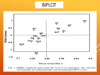
The document discusses the AMMI model for analyzing genotype by environment interactions in plant breeding experiments. It begins by introducing the concept of genotype by environment interaction and different models used for stability analysis. It then describes the AMMI model in detail, including that it combines ANOVA and PCA to analyze main and interaction effects. Key features of AMMI mentioned are that it identifies patterns of interaction, provides reliable genotype performance estimates, and enables visualization of relationships through biplots. Examples are given of crops AMMI has been applied to successfully.

1. SEMINAR TOPIC
AMMI MODEL FOR STABILITY ANALYSIS IN PLANT
BREEDING
PRESENTED BY,
Balaji S. Thorat
Ph. D. (Scholar)
GENETICS & PLANT BREEDING

2.  The challenge put forward for the plant breeder has been
to develop cultivars that are stable across a range of
environments. The goal of breeding stable genotypes may
be translated as the goal of minimizing genotype
environment interaction, which makes the selection of
high yielding genotypes easier
Introduction
In these experiments, changes in the relative behaviour
of the genotype in different environments are usually
observed. This phenomenon is called genotype by
environment interaction (GxE). It is the rule in most
quantitative characteristics (Bernardo, 2002).

3.  The GxE interaction makes it difficult to select genotypes
that produce high yields and that are more stable in
breeding programs. This, of course, reduces the selection
progress (Yan & Hunt, 1998).
 Genotypes respond differently across a range of
environments i.e., the relative performance of varieties
depends on the environment.

4.  The term stability refers to the ability of the
genotypes to be consistent, both with high or
low yield levels in various environments.
There are two basic concept of stability analysis .
1.Biological concept
2.Agronomical concept
Stability

5.  Adaptability refers to the adjustment of an organism
to its environment, e.g., a genotype that produces
high yields in specific environmental conditions and
poor yields in another environment (Balzarini et al.
2005).
Adaptability

6.  Combined ANOVA,
 Multivariate methods
 Stability analysis : An analysis to estimate
the adaptability of a genotype. It included
two model:
Different model for stability
analysis are given below :
Statistical methods to analyse the GxE
interaction :

7. A. Conventional model :
1.stability factor model.(Lewis1954)
2.ecovalence model.(Wricke1964)
3.stability variance model(Sukla1972)
4.lin and binns model.(1988)
B. Regression coefficient model :
1. Finley and Wilkinson model.(1963)
2.Eberhart and Russell model.(1966)
3.Perkins and Jinks model.(1968)
4.Freeman and Perkins model(1971)
C. Principal component analysis :
1.Additive Main effect and Multiplicative Interaction
(AMMI) model (Gauch 1992)

8. AMMI is a combination of ANOVA for the main
effects of the genotypes and the environment
together with principal components analysis (PCA)
the genotype-environment interaction (Zobel et al.
1998; Gauch, 1988).
AMMI models are usually called AMMI (1),
AMMI(2), ….,AMMI (n), depending on the number
of principal components used to study the
interaction and Graphical representations
obtained using biplots (Gabriel, 1971)
AMMI Model

9. The Additive Main effect and Multiplicative
Interaction (AMMI) method proposed by Gauch
(1992) is a statistical tool which leads to
identification of stable genotypes with their
adaptation behaviour in an easy manner.
AMMI first calculate genotype and environment
environment additive effect using analysis of
variance (ANOVA) and then analyse residual from
these model using principal components analysis
(PCA)

10. PCA compute a genotype score and environment
score whose product estimates the yield for that
genotype in that environment.
Those the result of AMMI equation is the least
square, which with further graphical representation
of the numerical result by using biplot analysis.

11. Yijl =  + Gi + Ej + (kikjk) + eijl
Where,
•Yij is the observed mean yield of the ith genotype in jth
environmt
•μ is the general mean
•Gi and Ej represent the effects of the genotype and
environment
•λk is the singular value of the kth axis in the PCA
•αik is the eigenvector of the ith genotype for the kth axis
•γjk is the eigenvector of the jth environment for the kth axis
•n is the number of principal components in the model
•eij is the average of the corresponding random errors
AMMI Model

12. source df SS MS F
TOTAL (ger- 1)
Treatment (ge -1)
Genotype (g -1)
Environment (e-1)
Interaction
IPCA 1
IPCA 2
Residual
(g-1) (e-1)
blocks (r-1)
error (r-1) (ge -1)
Analysis of variance for stability – AMMI Model

13. CROPS IN WHICH AMMI STABILITY ANALYSIS
CARRIED OUT
 The effectiveness of AMMI procedure has been clearly
demonstrated by various authors using multilocation
data in
 soybean (Zobel et al., 1998),
 maize (Crossa et al., 1990),
 Wheat (Ruzgas et al.2006),
 Pear millet (Shinde et al., 2002),
 Okra (Ariyo and Ayo-Vaughan 2000),
 Field pea (Taye et al., 2000)
 Rice (Islam et al., 2014).

14. MAIN FEATURE OF AMMI MODEL .
Method for analyzing GEI to identify patterns of
interaction.
Combines conventional ANOVA with principal
component analysis
May provide more reliable estimates of genotype
performance than the mean across sites

15. • Biplots help to visualize relationships among genotypes
and environments; show both main and interaction
effects.
• Enables you to identify target breeding environments
and to choose representative testing sites in those
environments.
• Enables you to select varieties with good adaptation to
target breeding environments.

16. Usually the first principal component (CP1)
represents responses of the genotypes that are
proportional to the environments, which are
associated with the GxE interaction.
The second principal component (CP2) provides
information about cultivation locations that are not
proportional to the environments, indicating that
those are responsible of the GxE crossover
interaction.
Principal components

17. Feature of PCA :
It computes a genotype score and an environment
score whose product estimate yield For that genotype
in that environment .

18. Graphical representation of interaction using AMMI
interaction parameters is known as biplot.
Till date, the stability conclusions made from AMMI
model are based on biplots. However the scope of
biplots is very much limited.
BIPLOTS
Biplot formulation of interaction will be successful
only when significant prop onion of G x E
interaction is concentrated in the first or first two
PCA axes.

19. Two kinds of plotting is possible with
estimated AMMI interaction parameters :
1.Biplot with First PCA Axis
• First PCA scores of genotypes and environments
are plotted against their respective means.
• Now the pattern of G x E interaction may be
visualized from this plot. If the genotype or an
environment has a PCA score of nearly zero, it
will have smaller interaction effects.

20. Biplot with First PCA Axis :

21. 2. Biplot with Two PCA Axis
• Here second PCA scores of genotypes and
environments are plotted against their respective
first PCA scores.
• For a better description of the interaction, both
first and second PCA scores of genotypes and
environments may be considered for plotting.

22. Objective:
To determine the adaptability and stability of
promising rice varieties.
CASE STUDY

25. BIPLOT

26. INFERENCE
 AMMI model is the most suitable to select high yielding hybrids for
specific as well as diverse environment.
 Almost all the genotypes were affected by G X E interaction.ie, no
genotype have superior performance.
 According to the AMMI biplot, four tested genotypes (G1, G2, G3 and
G4) were found to be best for E1 and E3 environment and
G7,G9,G10,G11&G12 most adapted to the environment E4, while G5 and
G8 not found best for any environment.

27. The AMMI analysis provided
1. A better understanding of the GEI through analysis of
variance.
2. It facilitated identification of genotypes possessing stable
yields as well as discriminating environments through the
biplot display.
3. Specificity in adaptability of the genotypes to specific
environments.
4. The scientific information obtained, could be of considerable
importance in developing location specific breeding strategies
and selecting stable genotypes in breeding programme.
27

28. Conclusion
The AMMI analysis provided a better
understanding of the GEI through analysis of
variance, facilitated identification of genotypes
possessing stable yields as well as
discriminating environments through the biplot
display and specificity in adaptability of the
genotypes to specific environments.

29. 29