This document provides an introduction to analysis of variance (ANOVA) and multivariate analysis of variance (MANOVA). It discusses key concepts like variance components, fixed and random models, and the assumptions of MANOVA. The goals of ANOVA are described as estimating variance components, evaluating genetic contributions, and testing hypotheses. MANOVA tests for differences in multiple dependent variables simultaneously, which can protect against Type I errors compared to multiple ANOVAs. Both methods require assumptions like normality and homogeneity of variances.

1. Welcome

2. Submitted To
Dr. S. D. Solanki,
Assistant Professor ,
Dept. of Genetics & Plant Breeding
C.P.C.A,S.D.A.U.,
Sardarkrushinagar.
Submitted By
Satish M. Khadia
Ph. D. , 6th sem.,
Dept. of Genetics & Plant Breeding
C.P.C.A,S.D.A.U.,
Sardarkrushinagar.
Course: GP 504 : Quantitative Genetics
An
Assignment on
Analysis of Variance (ANOVA), MANOVA: Expected
variance components, Random and fixed models

3. Introduction
• Variance: Average of the squares of deviations of the observations of a
sample from the mean of the sample drown from a population
[ ∑(x – x)2/N]
• Variance: The square of the standard deviation.
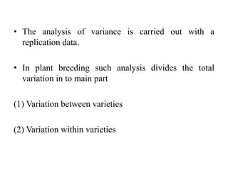
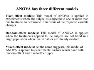
• The statistical procedure which separate or split the total variation into
different components is known as “ANOVA”
• R.A. Fisher
• “It is the technique of sorting out the total variation into some known and
unknown component of variation from a given set of data”
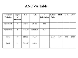
 Recognized source of variance are replication, genotype, error and total.
 It is a mathematical procedure of partitioning the total variation into various
recognized source of variance

4. Main Advantage
• Estimation of Components of Variance
• Provide basis for the test of significance

5. Aims of ANOVA
To sort out total variance and there by to
estimate variance components.
 To evaluate the hereditary contribution in a
genetically problem.
 To test predetermined hypothesis.

6. Scope of ANOVA
• Treatment study.
• Gives scope to understand treatment comparison.
• Gives idea of the magnetite of uncontrolled variation.
• It helps in future planning of experiment.
• It can be controlled by adopting principle of experimental
design.

7. • The data pertaining to various characters were
used for analysis of variance by using
following linear additive statistical model
(Panse and Sukhatme, 1978).
Yij = µ + ri + gj + eij

8. • Yij : Value of jth genotype in ith replication,
• µ : General mean,
• ri : Effect of ith replication,
• gj : Effect of jth genotype
• eij : Uncontrolled variation or random error associated
with jth genotype in ith replication.
Yij = µ + ri + gj + eij

9. Analysis of Variance
Source d.f. Sum of
square
Mean
square
E.M.S.
Replications (r) (r-1) RSS Mr σ2e + gσ 2r
Genotypes (g) (g-1) GSS Mg σ2e + rσ 2g
Error (r-1)(g-1) ESS Me σ 2e
Total (rg-1) TSS

10. Where,
r = Number of replications
g = Number of genotypes
σ 2e = Variance due to error
σ 2r = Variance due to replication
σ 2g = Variance due to genotype
M1, M2, M3=Mean squares for replication,
genotype and error, respectively.

11. • The analysis of variance is carried out with a
replication data.
• In plant breeding such analysis divides the total
variation in to main part
(1) Variation between varieties
(2) Variation within varieties

12. Variance Components
• Genotypic variance (σ 2g)
• Phenotypic variance (σ 2p)
• Error variance (σ 2e)

13. 1. Genotypic variance (σ 2g)
• The genotypic variance contributed by genetic causes or the
occurrence of differences among individuals due to differences
in their genetic make-up. It was calculated as under:
• Genotypic variance (σ 2g) = Mg – Me
--------
r
Where,
σ 2g = Genotypic variance,
Mg = Genotypic mean square of the character,
Me = Error mean square of the character, and
r = Number of replications.

14. 2. Phenotypic variance (σ 2p)
• It was sum of the variance contributed by genetic
causes and environmental factors. It was calculated
as under:
• Phenotypic variance (σ 2p)= σ 2g + σ 2e
Where,
• σ2p =Phenotypic variance
• σ 2g =Genotypic variance
• σ 2e =Error variance

15. 3. Error variance (σ 2e)
• The mean square of error represented by the variation
attributed to environmental causes.
Environmental variance (σ 2e)=Me
Where,
• Σ2e =Error variance,
• Me =Mean square due to error.

16. Coefficient of Variance
• Burton (1952)
ANOVA also permits the estimation of
• Phenotype Coefficient Of Variance(PCV)
• Genotype Coefficient Of Variance(GCV)
• Environmental Coefficient Of Variance(ECV)

17. • PCV % = σ 2p × 100
Mean
• GCV% = σ 2g × 100
Mean
• ECV% = σ 2e × 100
Mean

18. • PCV and GCV are classified for suggested by
• Shivsubramanium and Madhavmenon (1973)
Low : Less than 10%
Moderate : 10-20%
High : More than 20%

19. ANOVA has three different models
Fixed-effect models: This model of ANOVA is applied in
experiments where the subject is subjected to one or more than
one treatment to determine if the value of the response variable
changes.
Random-effect models: This model of ANOVA is applied
when the treatments applied to the subject are not fixed in a
large population where the variables are already random.
Mixed-effect models: As the name suggests, this model of
ANOVA is applied to experimental factors which have both
random-effect and fixed-effect types.

20. Fixed and Random Factors
In fixed effect model the experimental material includes a set of fixed
genotypes, say a set of inbreeds or varieties. Such set of genotype is considered as a
population and inferences are to be drawn on individual line/variety.
The model employed for fixed levels is called a fixed model.
In the random effect model, we deal with random sample of a population of
inbred lines. In this case the inferences are not to be drawn on individual lines in
the sample but about the parent population as a whole.
Model is called a random model

21. Properties of random effects
• To illustrate some of the properties of random effects,
suppose you collected data on the amount of insect
damage to different varieties of wheat.
• It is impractical to study insect damage for every
possible variety of wheat, so to conduct the
experiment, you randomly select four varieties of
wheat to study.
• Plant damage is rated for up to a maximum of four
plots per variety. Ratings are on a 0 (no damage) to
10 (great damage) scale.

22. DATA: wheat
VARIETY PLOT DAMAGE
A
A
A
B
B
B
B
C
C
C
C
D
D
1
2
3
4
5
6
7
8
9
10
11
12
13
3.90
4.05
4.25
3.60
4.20
4.05
3.85
4.15
4.60
4.15
4.40
3.35
3.80

23. • To determine the components of variation in
resistance to insect damage for Variety and Plot, an
ANOVA can first be performed. Perhaps surprisingly,
in the ANOVA, Variety can be treated as a fixed
effect and Plot as a random effect.

24. ANOVA results for this mixed model & random effect
analysis
ANOVA Results for Synthesized Errors: DAMAGE (wheat)
df error computed using Satterthwaite method
Effect
Effect
(F/R)
df
Effect
MS
Effect
df
Error
MS
Error F p
Variety
Plot
Fixed
Random
3
9
.270053
.056435
9
-----
.056435
-----
4.785196
-----
.029275
-----

25. • The difference in the two sets of estimates is that a variance
component is estimated for Variety only when it is considered
to be a random effect.
• This reflects the basic distinction between fixed and random
effects.
• The variation in the levels of random factors is assumed to be
representative of the variation of the whole population of
possible levels.
• Thus, variation in the levels of a random factor can be used to
estimate the population variation.
• Thus, the variation of a fixed factor cannot be used to estimate
its population variance, nor can the population covariance with
the dependent variable be meaningfully estimated.

26. Multivariate Analysis of Variance
(MANOVA)

27.  Multivariate analysis of variance (MANOVA) is simply an
ANOVA with several dependent variables .
 That is to say, ANOVA tests for the difference in means between
two or more groups, while MANOVA tests for the difference in
two or more vectors of means.
 There are two major situations in which MANOVA is used.
 The first is when there are several correlated dependent variables,
and the researcher desires a single, overall statistical test on this set
of variables instead of performing multiple individual tests.
 The second, and in some cases, the more important purpose is to
explore how independent variables influence some patterning of
response on the dependent variables.

28. For e.g.
 In many agricultural experiment, the data on more than one
character is observed. One common e.g. is grain yield & straw yield.
 The analysis normally done only on grain yield & the best treatment
is identified on the basis of this character alone.
 The straw yield is generally not taken into account.
 But the straw yield also important for cattle feed or mulching.
 So in these situations Multivariate Analysis of Variance can be
helpful.

29.  MANOVA is useful in experimental situations where at
least some of the independent variables are manipulated.
 It has several advantages over ANOVA.
 First, by measuring several dependent variables in a
single experiment, there is a better chance of discovering
which factor is truly important.
 Second, it can protect against Type I errors that might
occur if multiple ANOVA’s were conducted
independently. Additionally, it can reveal differences not
discovered by ANOVA tests.

30.  These are the assumptions should be taken by observer
during study of MANOVA.
1) Normal Distribution: The dependent variable should be
normally distributed within groups.
2) Linearity: MANOVA assumes that there are linear
relationships among all pairs of dependent variables.
3) Homogeneity of Variances: Homogeneity of variances
assumes that the dependent variables exhibit equal levels of
variance across the range of predictor variables.
4) Homogeneity of Variances and Covariances: In multivariate
designs, with multiple dependent measures, the homogeneity of
variances assumption described earlier also applies.

31. Limitations
 Outliers - Like ANOVA, MANOVA is extremely sensitive to outliers.
Outliers may produce either a Type I or Type II error and give no
indication as to which type of error is occurring in the analysis. There
are several programs available to test for univariate and multivariate
outliers.
 Multicollinearity and Singularity - When there is high correlation
between dependent variables, one dependent variable becomes a near-
linear combination of the other dependent variables. Under such
circumstances, it would become statistically redundant and suspect to
include both combinations

32. The procedure for the analysis of the variance remains the
same in both the models, but the expectations of mean squares due
to various items are different and therefore, the interpretation of
results also differs.
This models are used for analysis of Combining Ability - Griffings-1956

33. Example 1. The yield of 6 varieties of a Wheat in kg./ plot are
given in following table. The experiment was conducted using
randomized block design with 5 replication.
Treatment Replication Treatment
Total
Treatment
Mean
1 2 3 4 5
V1 20 26 30 28 23 127 25.40
V2 09 12 16 16 07 54 10.80
V3 12 15 14 14 14 71 14.20
V4 17 10 23 23 20 90 18.00
V5 28 26 35 35 30 140 28.40
V6 40 50 64 64 70 280 56.00
Total 126 139 180 180 164 764 25.46

34. 1.General Mean =
2.Correction Factor =
= 19456.53
Analysis of variance

35. 3.Total SS = (individual observation)² - C.F.
=(20)²+(9)²+(12)²+……..+(70)² – 19456.53
=27000 – 19456.53
= 7543.47
4.Treatment SS =
=

36. 5.Replication SS =
=
= 19753 - 19456.53
= 296.47
6.Error SS = Total ss. - treatment ss. - replication ss.
= 7543.47 - 6693.47 - 296.47
= 553.53

37. 7. Mean Square treatment =
8. Mean Square Error =
=
= 27.67

38. 9. F. Calculated =
=
10. Critical difference = SEM × × Table value of 0.05
= 2.35 × 1.41 × 2.131
= 7.06

39. 11. Standard error of mean =
12. Coefficient of variation =
= 20.66
(C V %)

40. Source of
Variation
Degree
of
Freedom
S. S. M. S. F.
Calculation
F. Table
Value
SEM C. D. C V%
Treatment 4 296.47 74.117 2.68
Replication 5 6693.47 1338.693 48.38
Error 20 553.53 27.67 2.137 2.35 7.06 20.66
Total 29 7543.47 1440.48
ANOVA Table

41. Advantages:
In this design more then one units can be used to one or
some treatment in each replication.
In the statistical analysis, even when more then one
units are used to a treatment per replication remains
simpler.
Any no. of treatment can be tried in this design
however this depends upon the homogeneity of the
material within a group of the replication.

42. Disadvantage:
If the grouping does not assure complete elimination of
heterogeneity among experimental units requires further
grouping and ultimately this design is less efficient.
If the observations are missing one has to estimate the
missing observations and then analyses the data. If large
no. of observations are missing one may be even able to
analysis the data.

43. References
• Falconer DS & Mackay J. 1998. Introduction to Quantitative Genetics. Longman.
• Mather K & Jinks JL. 1971. Biometrical Genetics. Chapman & Hall.
• Naryanan SS & Singh P. 2007. Biometrical Techniques in Plant Breeding. Kalyani.

44. THANK YOU