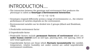
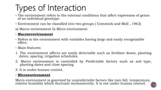
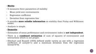
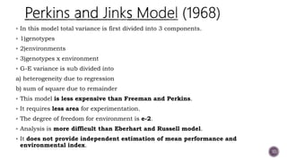
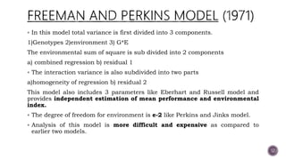
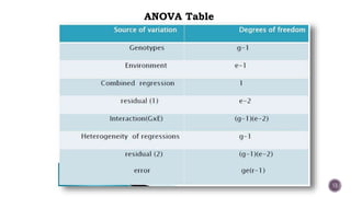
Models in stability analysis
Presented By:
MAYUR KUMAR SONAGARA
Reg No. – 1010119017
Ph.D. Scholar (1st Sem)
Genetics And Plant Breeding
AAU, Anand.
Submitted To:
Dr. M. P. PATEL
Assistant Research Scientist (Pl. Br.)
Regional Research Station,
AAU, Anand.
1
 The interaction between the genotype and environment that produces the
phenotype is called as Genotype x Environmental Interaction.
 P = G + E + G×E
 Genotypes respond differently across a range of environments i.e., the relative
performance of varieties depends on the environment.
 Environmental variable can be divided into 2 groups (Allard and Bradshaw,
1964)
1.Predictable environment factor
2.Unpredictable factor
 Predictable factors include permanent features of environment which are
under human control such as soil type, planting date, row spacing, rows of
new trend application.
 Unpredictable factors are those which fluctuate inconsistently like rainfall,
temperature, relative humidity not under control are called unpredictable
environment conditions. 2
 The environment refers to the external conditions that affect expression of genes
of an individual genotype.
 Environment can be classified into two groups ( Comstock and Moll , 1963)
a) Macro environment b) Micro environment
 Macroevnvironment
 Refers to the environment with variables having large and easily recognizable
effect.
 Main features:
1. The environment affects are easily detectable such as fertilizer doses, planting
dates, spacing, irrigation schedules.
2. Macro environment is controlled by Predictable factors such as soil type,
planting dates and close spacing.
3. It is under human control.
 Microenvironment
Micro environment is governed by unpredictable factors like rain fall, temperature,
relative humidity which fluctuate inconsistently. It is not under human control. 3
 Stability refers to the performance with respective changing
environmental factors overtime within given location.
 Selection for stability is not possible until a biometrical model with suitable
parameters is available to provide criteria necessary to rank varieties /
breeds for stability.
 Low magnitude of G.E interaction involves the consistent performance of a
population over variable environments.
 It consists of following steps: Location / environment wise analysis of
variance. Pooled analysis of variance for all the locations/ environments.
 If G.E interaction is found significant, stability analysis can be carried out
using one of the four methods:
1.Finlay and Wilkinson model (1963)
2.Eberhat and Russell model (1966)
3.Perkins and Jinks model (1968)
4.Freeman and Perkins model (1971)
4
 Used two parameters 1)Mean performance over environments. 2)Regression
performance in different environments.
 The following inferences can be drawn:
1)The regression coefficient of unity indicates average stability .
2)If the regression coefficient is >1,it means below average stability .
3) If the regression coefficient is <1, it means above average stability.
4) Regression coefficient of 0 would express absolute stability.
MERITS
1. Analysis of this model is simple.
2. Parameters- mean yield over locations and regression coefficient are used to asses
the phenotypic stability.
DEMERITS
1. The deviations from the regression line are not estimated which are important for
the stability analysis.
2. Greater emphasis is given on mean performance over environments than regression
coefficients.
5
 It is the most popular and useful model.
 In 1966 both made further improvement in stability analysis by partitioning the
G.E interaction of each variety into 2 parts. one is slope of the regression line ,
second is deviation from regression line.
 In this model total variance is first divided into 2 components:
 genotypes
 environment plus interaction (E+G*E).
 The second component is further divided in to 3 components.
I. Environment linear
II. G.E linear
III. Pooled deviations
 Sum of squares due to pooled deviations are further divided into sum of squares
due to individual genotype.
6
Main Features of this Model:
This model consists of three parameters
a) Mean yield over locations
b) Regression coefficient =bi
c) Deviation from regression =s²di
 Analysis of stability parameters is simple as compared to other models of stability
analysis.
 The degree of freedom for environment is 1.
 It requires less area hence less expensive when compared to other models.
 It does not provide independent estimation for mean performance and
environmental index.
7
8
ANOVA Table
Merits:
 It measures three parameters of stability
1. Mean yield over environments
2. Regression coefficient
3. Deviation from regression line
 It provides more reliable information on stability than Finlay and Wilkinson
model.
 Analysis is simple.
Demerits:
 Estimation of mean performance and environment index is not independent.
 There is a combined estimation of sum of squares of environment and
interactions which is not proper.
 Eberhart and Russell (1956) defined stable variety as one with a regression
coefficient of unity(b=1) and a minimum deviation from the regression
lines(s²d=0).
9
 In this model total variance is first divided into 3 components.
 1)genotypes
 2)environments
 3)genotypes x environment
 G-E variance is sub divided into
a) heterogeneity due to regression
b) sum of square due to remainder
 This model is less expensive than Freeman and Perkins.
 It requires less area for experimentation.
 The degree of freedom for environment is e-2.
 Analysis is more difficult than Eberhart and Russell model.
 It does not provide independent estimation of mean performance and
environmental index.
10
11
ANOVA Table
 In this model total variance is first divided into 3 components.
1)Genotypes 2)environment 3) G*E
The environmental sum of square is sub divided into 2 components
a) combined regression b) residual 1
 The interaction variance is also subdivided into two parts
a)homogeneity of regression b) residual 2
This model also includes 3 parameters like Eberhart and Russell model and
provides independent estimation of mean performance and environmental
index.
 The degree of freedom for environment is e-2 like Perkins and Jinks model.
 Analysis of this model is more difficult and expensive as compared to
earlier two models.
12
13
ANOVA Table
14

Stability models

  • 1.
    Models in stabilityanalysis Presented By: MAYUR KUMAR SONAGARA Reg No. – 1010119017 Ph.D. Scholar (1st Sem) Genetics And Plant Breeding AAU, Anand. Submitted To: Dr. M. P. PATEL Assistant Research Scientist (Pl. Br.) Regional Research Station, AAU, Anand. 1
  • 2.
     The interactionbetween the genotype and environment that produces the phenotype is called as Genotype x Environmental Interaction.  P = G + E + G×E  Genotypes respond differently across a range of environments i.e., the relative performance of varieties depends on the environment.  Environmental variable can be divided into 2 groups (Allard and Bradshaw, 1964) 1.Predictable environment factor 2.Unpredictable factor  Predictable factors include permanent features of environment which are under human control such as soil type, planting date, row spacing, rows of new trend application.  Unpredictable factors are those which fluctuate inconsistently like rainfall, temperature, relative humidity not under control are called unpredictable environment conditions. 2
  • 3.
     The environmentrefers to the external conditions that affect expression of genes of an individual genotype.  Environment can be classified into two groups ( Comstock and Moll , 1963) a) Macro environment b) Micro environment  Macroevnvironment  Refers to the environment with variables having large and easily recognizable effect.  Main features: 1. The environment affects are easily detectable such as fertilizer doses, planting dates, spacing, irrigation schedules. 2. Macro environment is controlled by Predictable factors such as soil type, planting dates and close spacing. 3. It is under human control.  Microenvironment Micro environment is governed by unpredictable factors like rain fall, temperature, relative humidity which fluctuate inconsistently. It is not under human control. 3
  • 4.
     Stability refersto the performance with respective changing environmental factors overtime within given location.  Selection for stability is not possible until a biometrical model with suitable parameters is available to provide criteria necessary to rank varieties / breeds for stability.  Low magnitude of G.E interaction involves the consistent performance of a population over variable environments.  It consists of following steps: Location / environment wise analysis of variance. Pooled analysis of variance for all the locations/ environments.  If G.E interaction is found significant, stability analysis can be carried out using one of the four methods: 1.Finlay and Wilkinson model (1963) 2.Eberhat and Russell model (1966) 3.Perkins and Jinks model (1968) 4.Freeman and Perkins model (1971) 4
  • 5.
     Used twoparameters 1)Mean performance over environments. 2)Regression performance in different environments.  The following inferences can be drawn: 1)The regression coefficient of unity indicates average stability . 2)If the regression coefficient is >1,it means below average stability . 3) If the regression coefficient is <1, it means above average stability. 4) Regression coefficient of 0 would express absolute stability. MERITS 1. Analysis of this model is simple. 2. Parameters- mean yield over locations and regression coefficient are used to asses the phenotypic stability. DEMERITS 1. The deviations from the regression line are not estimated which are important for the stability analysis. 2. Greater emphasis is given on mean performance over environments than regression coefficients. 5
  • 6.
     It isthe most popular and useful model.  In 1966 both made further improvement in stability analysis by partitioning the G.E interaction of each variety into 2 parts. one is slope of the regression line , second is deviation from regression line.  In this model total variance is first divided into 2 components:  genotypes  environment plus interaction (E+G*E).  The second component is further divided in to 3 components. I. Environment linear II. G.E linear III. Pooled deviations  Sum of squares due to pooled deviations are further divided into sum of squares due to individual genotype. 6
  • 7.
    Main Features ofthis Model: This model consists of three parameters a) Mean yield over locations b) Regression coefficient =bi c) Deviation from regression =s²di  Analysis of stability parameters is simple as compared to other models of stability analysis.  The degree of freedom for environment is 1.  It requires less area hence less expensive when compared to other models.  It does not provide independent estimation for mean performance and environmental index. 7
  • 8.
  • 9.
    Merits:  It measuresthree parameters of stability 1. Mean yield over environments 2. Regression coefficient 3. Deviation from regression line  It provides more reliable information on stability than Finlay and Wilkinson model.  Analysis is simple. Demerits:  Estimation of mean performance and environment index is not independent.  There is a combined estimation of sum of squares of environment and interactions which is not proper.  Eberhart and Russell (1956) defined stable variety as one with a regression coefficient of unity(b=1) and a minimum deviation from the regression lines(s²d=0). 9
  • 10.
     In thismodel total variance is first divided into 3 components.  1)genotypes  2)environments  3)genotypes x environment  G-E variance is sub divided into a) heterogeneity due to regression b) sum of square due to remainder  This model is less expensive than Freeman and Perkins.  It requires less area for experimentation.  The degree of freedom for environment is e-2.  Analysis is more difficult than Eberhart and Russell model.  It does not provide independent estimation of mean performance and environmental index. 10
  • 11.
  • 12.
     In thismodel total variance is first divided into 3 components. 1)Genotypes 2)environment 3) G*E The environmental sum of square is sub divided into 2 components a) combined regression b) residual 1  The interaction variance is also subdivided into two parts a)homogeneity of regression b) residual 2 This model also includes 3 parameters like Eberhart and Russell model and provides independent estimation of mean performance and environmental index.  The degree of freedom for environment is e-2 like Perkins and Jinks model.  Analysis of this model is more difficult and expensive as compared to earlier two models. 12
  • 13.
  • 14.