Chapter24rev1.pptPart 6Chapter 24Boundary-Valu.docx

Chapter24rev1.ppt
Part 6
Chapter 24
Boundary-Value Problems
PowerPoints organized by Dr. Michael R. Gustafson II, Duke
University
All images copyright © The McGraw-Hill Companies, Inc.
Permission required for reproduction or display.
Chapter ObjectivesUnderstanding the difference between initial-
value and boundary-value problems.Knowing how to express an
nth order ODE as a system of n first-order ODEs.Knowing how
to implement the shooting method for linear ODEs by using
linear interpolation to generate accurate “shots.”Understanding
how derivative boundary conditions are incorporated into the
shooting method.
Objectives (cont)Knowing how to solve nonlinear ODEs with
the shooting method by using root location to generate accurate
“shots.”Knowing how to implement the finite-difference
method.Understanding how derivative boundary conditions are
incorporated into the finite-difference method.Knowing how to
solve nonlinear ODEs with the finite-difference method by

using root location methods for systems of nonlinear algebraic
equations.
Boundary-Value ProblemsBoundary-value problems are those
where conditions are not known at a single point but rather are
given at different values of the independent variable.Boundary
conditions may include values for the variable or values for
derivatives of the variable.
Copyright © The McGraw-Hill Companies, Inc. Permission
required for reproduction or display.
Higher Order SystemsMATLAB’s ODE solvers are based on
solving first-order differential equations only.To solve an nth
order system (n>1), the system must be written as n first-order
equations:
Each first-order equation needs an initial value or boundary
value to solve.
The Shooting MethodOne method for solving boundary-value
problems - the shooting method - is based on converting the
boundary-value problem into an equivalent initial-value
problem.Generally, the equivalent system will not have
sufficient initial conditions and so a guess is made for any
undefined values.The guesses are changed until the final
solution satisfies all the boundary conditions.For linear ODEs,
only two “shots” are required - the proper initial condition can
be obtained as a linear interpolation of the two guesses.

Copyright © The McGraw-Hill Companies, Inc. Permission
required for reproduction or display.
Boundary ConditionsDirichlet boundary conditions are those
where a fixed value of a variable is known at a particular
location.Neumann boundary conditions are those where a
derivative is known at a particular location.Shooting methods
can be used for either kind of boundary condition.
The Shooting Method for Nonlinear ODEsFor nonlinear ODEs,
interpolation between two guesses will not necessarily result in
an accurate estimate of the required boundary condition.Instead,
the boundary condition can be used to write a roots problem
with the estimate as a variable.
ExampleSolve
-9 K-3 m-2, L=10 m, h’=0.05 m-
T(0) = 300 K, and T(10) = 400 K.First - break into two
equations:
Example CodeCode for derivatives:

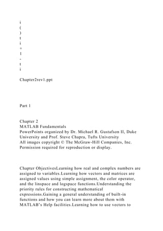
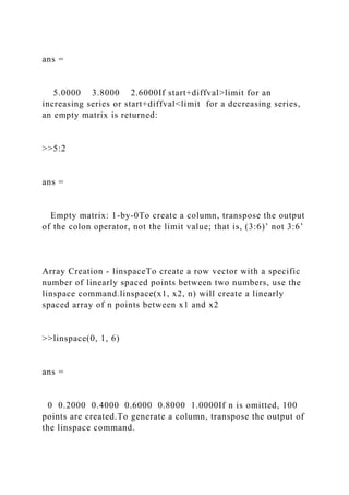
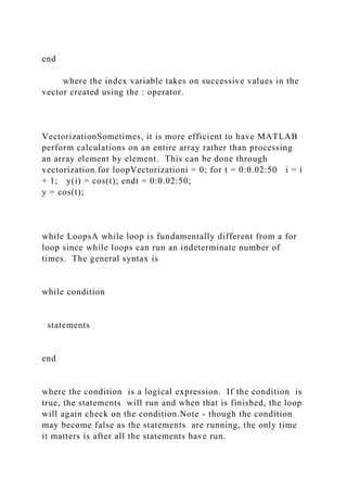
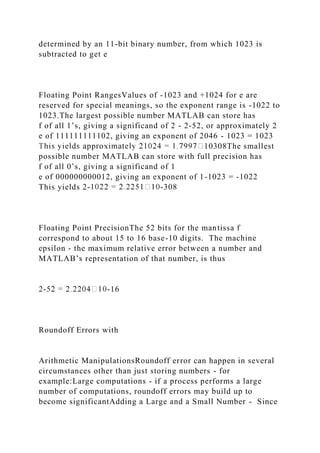
function dy=dydxn(x,y)
dy=[y(2);…
-0.05*(200-y(1))-2.7e-9*(1.6e9-y(1)^4)];Code for residual:
function r=res(za)
[x,y]=ode45(@dydxn, [0 10], [300 za]);
r=y(length(x),1)-400;Code for finding root of residual:
fzero(@res, -50) Code for solving system:
[x,y]=ode45(@dydxn, [0 10], [300 fzero(@res, -50) ]);
Finite-Difference MethodsThe most common alternatives to the
shooting method are finite-difference approaches.In these
techniques, finite differences are substituted for the derivatives
in the original equation, transforming a linear differential
equation into a set of simultaneous algebraic equations.
Finite-Difference ExampleConvert:

into n-1 simultaneous equations at each interior point using
centered difference equations:
Finite-Difference Example (cont)Since T0 and Tn are known,
they will be on the right-hand-side of the linear algebra system
(in this case, in the first and last entries, respectively):
Derivative Boundary ConditionsNeumann boundary conditions
are resolved by solving the centered difference equation at the
point and rewriting the system equation accordingly.For
example, if there is a Neumann condition at the T0 point,
Finite-Difference Method for Nonlinear ODEsRoot location
methods for systems of equations may be used to solve
nonlinear ODEs.Another method is to adapt a successive
substitution algorithm to calculate the values of the interior
points.
d
2
T
dx

2
+
¢
h
T
¥
-
T
(
)
=
0
Þ
dT
dx
=
z
dT
dz
=
-
¢
h
T
¥
-
T
(
)
ì
í
ï
î
ï
d

2
T
dx
2
+
¢
h
T
¥
-
T
(
)
+
¢
s
T
¥
4
-
T
4
(
)
=
0
d
2
T
dx
2
+
¢
h
T

¥
-
T
(
)
+
¢
s
T
¥
4
-
T
4
(
)
=
0
Þ
dT
dx
=
z
dT
dz
=
-
0
.
05
200
-
T
(
)
-

2
.
7
´
10
-
9
1
.
6
´
10
9
-
T
(
)
ì
í
ï
î
ï
d
2
T
dx
2
+
¢
h
T
¥
-
T
(

)
=
0
dT
dx
0
=
T
1
-
T
-
1
2
D
x
Þ
T
-
1
=
T
1
-
2
D
x
dT
dx
0
æ
è
ç
ö
ø

÷
-
T
-
1
+
2
+
¢
h
D
x
2
(
)
T
0
-
T
1
=
¢
h
D
x
2
T
¥
-
T
1
-
2
D
x
dT

dx
0
æ
è
ç
ö
ø
÷
é
ë
ê
ù
û
ú
+
2
+
¢
h
D
x
2
(
)
T
0
-
T
1
=
¢
h
D
x
2
T

¥
2
+
¢
h
D
x
2
(
)
T
0
-
2
T
1
=
¢
h
D
x
2
T
¥
-
2
D
x
dT
dx
0
æ
è
ç
ö
ø

÷
d
2
T
dx
2
=
T
i
-
1
-
2
T
i
+
T
i
+
1
D
x
2
T
i
-
1
-
2
T
i
+
T
i
+

1
D
x
2
+
¢
h
T
¥
-
T
i
(
)
=
0
-
T
i
-
1
+
2
+
¢
h
D
x
2
(
)
T
i
-
T
i

+
1
=
¢
h
D
x
2
T
¥
2
+
¢
h
D
x
2
-
1
-
1
2
+
¢
h
D
x
2
-
1
O
O
O
-

1
2
+
¢
h
D
x
2
é
ë
ê
ê
ê
ê
ù
û
ú
ú
ú
ú
T
1
T
2
M
T
n
-
1
ì
í
ï
î
ï
ü
ý

ï
þ
ï
=
¢
h
D
x
2
T
¥
+
T
0
¢
h
D
x
2
T
¥
M
¢
h
D
x
2
T
¥
+
T
n
ì
í
ï
ï

î
ï
ï
ü
ý
ï
ï
þ
ï
ï
Chapter1rev1.ppt
Part 1
Chapter 1
Mathematical Modeling,
Numerical Methods,
and Problem Solving
University and Prof. Steve Chapra, Tufts University
Chapter ObjectivesLearning how mathematical models can be
formulated on the basis of scientific principles to simulate the

behavior of a simple physical system.Understanding how
numerical methods afford a means to generalize solutions in a
manner that can be implemented on a digital
computer.Understanding the different types of conservation
laws that lie beneath the models used in the various engineering
disciplines and appreciating the difference between steady-state
and dynamic solutions of these models.Learning about the
different types of numerical methods we will cover in this book.
A Simple Mathematical ModelA mathematical model can be
broadly defined as a formulation or equation that expresses the
essential features of a physical system or process in
mathematical terms.Models can be represented by a functional
relationship between dependent variables, independent
variables, parameters, and forcing functions.
Model Function
Dependent variable - a characteristic that usually reflects the
behavior or state of the system Independent variables -
dimensions, such as time and space, along which the system’s
behavior is being determined Parameters - constants reflective
of the system’s properties or composition Forcing functions -
external influences acting upon the system
Model Function ExampleAssuming a bungee jumper is in mid-
flight, an analytical model for the jumper’s velocity, accounting
for drag, is

Dependent variable - velocity vIndependent variables - time
tParameters - mass m, drag coefficient cdForcing function -
gravitational acceleration g
Model ResultsUsing a computer (or a calculator), the model can
be used to generate a graphical representation of the system.
For example, the graph below represents the velocity of a 68.1
kg jumper, assuming a drag coefficient of 0.25 kg/m
Numerical ModelingSome system models will be given as
implicit functions or as differential equations - these can be
solved either using analytical methods or numerical
methods.Example - the bungee jumper velocity equation from
before is the analytical solution to the differential equation
where the change in velocity is determined by the gravitational
forces acting on the jumper versus the drag force.
Numerical MethodsTo solve the problem using a numerical
method, note that the time rate of change of velocity can be
approximated as:

Euler's MethodSubstituting the finite difference into the
differential equation gives
Solve for
Numerical ResultsApplying Euler's method in 2 s intervals
yields:
How do we improve the solution?Smaller steps
Bases for Numerical ModelsConservation laws provide the
foundation for many model functions. Different fields of
engineering and science apply these laws to different paradigms
within the field.Among these laws are:
Conservation of mass
Conservation of momentum
Conservation of charge
Conservation of energy

Summary of Numerical MethodsThe book is divided into five
categories of numerical methods:
Dependent
variable
=
f
independent
variables
,
parameters,
forcing
functions
æ
è
ç
ö
ø
÷
v
t
(
)
=
gm
c
d
tanh
gc
d
m
t

æ
è
ç
ö
ø
÷
dv
dt
=
g
-
c
d
m
v
2
dv
dt
»
D
v
D
t
=
v
t
i
+
1
(
)
-
v
t

i
(
)
t
i
+
1
-
t
i
Chapter2rev1.ppt
Part 1
Chapter 2
MATLAB Fundamentals
Chapter ObjectivesLearning how real and complex numbers are
assigned to variables.Learning how vectors and matrices are
assigned values using simple assignment, the color operator,
and the linspace and logspace functions.Understanding the
priority rules for constructing mathematical
expressions.Gaining a general understanding of built-in
functions and how you can learn more about them with
MATLAB’s Help facilities.Learning how to use vectors to

create a simple line plot based on an equation.
The MATLAB EnvironmentMATLAB uses three primary
windows-
Command window - used to enter commands and data
Graphics window(s) - used to display plots and graphics
Edit window - used to create and edit M-files
(programs)Depending on your computer platform and the
version of MATLAB used, these windows may have different
looks and feels.
Calculator ModeThe MATLAB command widow can be used as
a calculator where you can type in commands line by line.
Whenever a calculation is performed, MATLAB will assign the
result to the built-in variable ansExample:
>> 55 - 16
ans =
39
MATLAB VariablesWhile using the ans variable may be useful
for performing quick calculations, its transient nature makes it
less useful for programming.MATLAB allows you to assign
values to variable names. This results in the storage of values
to memory locations corresponding to the variable

name.MATLAB can store individual values as well as arrays; it
can store numerical data and text (which is actually stored
numerically as well).MATLAB does not require that you pre-
initialize a variable; if it does not exist, MATLAB will create it
for you.
ScalarsTo assign a single value to a variable, simply type the
variable name, the = sign, and the value:
>> a = 4
a =
4Note that variable names must start with a letter, though they
can contain letters, numbers, and the underscore (_) symbol
Scalars (cont)You can tell MATLAB not to report the result of a
calculation by appending the semi-solon (;) to the end of a line.
The calculation is still performed.You can ask MATLAB to
report the value stored in a variable by typing its name:
>> a
a =
4

Scalars (cont)You can use the complex variable i (or j) to
represent the unit imaginary number.You can tell MATLAB to
report the values back using several different formats using the
format command. Note that the values are still stored the same
way, they are just displayed on the screen differently. Some
examples are:short - scaled fixed-point format with 5 digitslong
- scaled fixed-point format with 15 digits for double and 7
digits for singleshort eng - engineering format with at least 5
digits and a power that is a multiple of 3 (useful for SI prefixes)
Format Examples>> format short; pi
ans =
3.1416
>> format long; pi
ans =
3.14159265358979
>> format short eng; pi

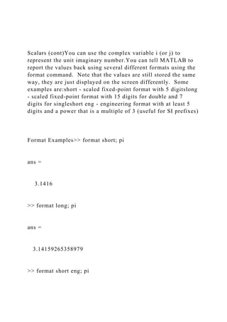
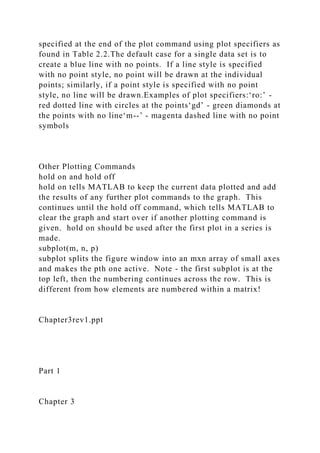
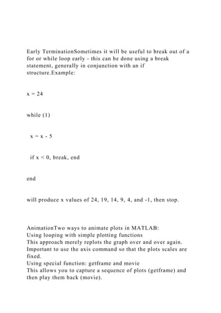
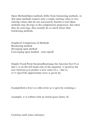
ans =
3.1416e+000
>> pi*10000
ans =
31.4159e+003Note - the format remains the same unless
another format command is issued.
Arrays, Vectors, and MatricesMATLAB can automatically
handle rectangular arrays of data - one-dimensional arrays are
called vectors and two-dimensional arrays are called
matrices.Arrays are set off using square brackets [ and ] in
MATLABEntries within a row are separated by spaces or
commasRows are separated by semicolons
Array Examples>> a = [1 2 3 4 5 ]
a =
1 2 3 4 5
>> b = [2;4;6;8;10]

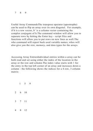
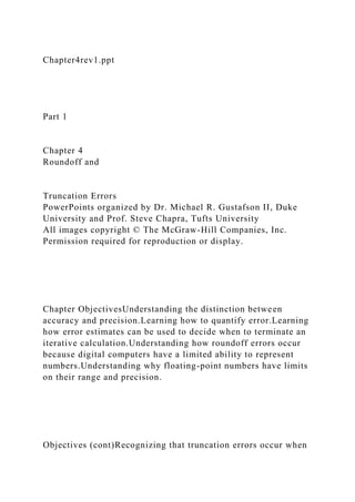
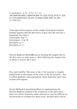
b =
2
4
6
8
10Note 1 - MATLAB does not display the bracketsNote 2 - if
you are using a monospaced font, such as Courier, the displayed
values should line up properly
MatricesA 2-D array, or matrix, of data is entered row by row,
with spaces (or commas) separating entries within the row and
semicolons separating the rows:
>> A = [1 2 3; 4 5 6; 7 8 9]
A =
1 2 3
4 5 6

7 8 9
Useful Array CommandsThe transpose operator (apostrophe)
can be used to flip an array over its own diagonal. For example,
if b is a row vector, b’ is a column vector containing the
complex conjugate of b.The command window will allow you to
separate rows by hitting the Enter key - script files and
functions will allow you to put rows on new lines as well.The
who command will report back used variable names; whos will
also give you the size, memory, and data types for the arrays.
Accessing Array EntriesIndividual entries within a array can be
both read and set using either the index of the location in the
array or the row and column.The index value starts with 1 for
the entry in the top left corner of an array and increases down a
column - the following shows the indices for a 4 row, 3 column
matrix:
1 5 9
2 6 10
3 7 11
4 8 12

Accessing Array Entries (cont)Assuming some matrix C:
C =
2 4 9
3 3 16
3 0 8
10 13 17C(2) would report 3C(4) would report 10C(13)
would report an error!Entries can also be access using the row
and column:C(2,1) would report 3C(3,2) would report 0C(5,1)
would report an error!
Array Creation - Built InThere are several built-in functions to
create arrays:zeros(r,c) will create an r row by c column matrix
of zeroszeros(n) will create an n by n matrix of zerosones(r,c)
will create an r row by c column matrix of onesones(n) will
create an n by n matrix one oneshelp elmat has, among other
things, a list of the elementary matrices
Array Creation - Colon OperatorThe colon operator : is useful
in several contexts. It can be used to create a linearly spaced
array of points using the notation

start:diffval:limit
where start is the first value in the array, diffval is the
difference between successive values in the array, and limit is
the boundary for the last value (though not necessarily the last
value).
>>1:0.6:3
ans =
1.0000 1.6000 2.2000 2.8000
Colon Operator - NotesIf diffval is omitted, the default value is
1:
>>3:6
ans =
3 4 5 6To create a decreasing series, diffval must be
negative:
>> 5:-1.2:2

ans =
5.0000 3.8000 2.6000If start+diffval>limit for an
increasing series or start+diffval<limit for a decreasing series,
an empty matrix is returned:
>>5:2
ans =
Empty matrix: 1-by-0To create a column, transpose the output
of the colon operator, not the limit value; that is, (3:6)’ not 3:6’
Array Creation - linspaceTo create a row vector with a specific
number of linearly spaced points between two numbers, use the
linspace command.linspace(x1, x2, n) will create a linearly
spaced array of n points between x1 and x2
>>linspace(0, 1, 6)
ans =
0 0.2000 0.4000 0.6000 0.8000 1.0000If n is omitted, 100
points are created.To generate a column, transpose the output of
the linspace command.

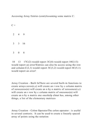
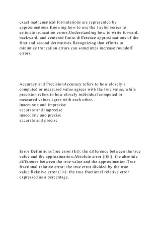
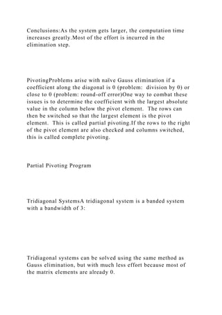
Array Creation - logspaceTo create a row vector with a specific
number of logarithmically spaced points between two numbers,
use the logspace command.logspace(x1, x2, n) will create a
logarithmically spaced array of n points between 10x1 and 10x2
>>logspace(-1, 2, 4)
ans =
0.1000 1.0000 10.0000 100.0000If n is omitted, 100 points
are created.To generate a column, transpose the output of the
logspace command.
Character Strings & EllipsisAlphanumeric constants are
enclosed by apostrophes (')
>> f = 'Miles ';
>> s = 'Davis'Concatenation: pasting together of strings
>> x = [f s]
x =
Miles DavisEllipsis (...): Used to continue long lines
>> a = [1 2 3 4 5 ...
6 7 8]
a =
1 2 3 4 5 6 7 8You cannot use an ellipsis
within single quotes to continue a string. But you can piece
together shorter strings with ellipsis
>> quote = ['Any fool can make a rule,' ...
' and any fool will mind it']
quote =

Any fool can make a rule, and any fool will mind it
Mathematical OperationsMathematical operations in MATLAB
can be performed on both scalars and arrays.The common
operators, in order of priority, are:^Exponentiation4^2 = 8-
Negation (unary operation)-8 = -8* /Multiplication and
Division2*pi = 6.2832 pi/4 = 0.7854Left Division62 = 0.3333
+ -Addition and Subtraction3+5 = 8 3-5 = -2
Order of OperationsThe order of operations is set first by
parentheses, then by the default order given above:
y = -4 ^ 2 gives y = -16
since the exponentiation happens first due to its higher default
priority, but
y = (-4) ^ 2 gives y = 16
since the negation operation on the 4 takes place first
Complex NumbersAll the operations above can be used with
complex quantities (i.e. values containing an imaginary part
entered using i or j and displayed using i)
>> x = 2+i*4; (or 2+4i, or 2+j*4, or 2+4j)
>> y = 16;
>> 3 * x

ans =
6.0000 +12.0000i
>> x+y
ans =
18.0000 + 4.0000i
>> x'
ans =
2.0000 - 4.0000i
Vector-Matrix CalculationsMATLAB can also perform
operations on vectors and matrices.The * operator for matrices
is defined as the outer product or what is commonly called
“matrix multiplication.”
The number of columns of the first matrix must match the
number of rows in the second matrix.
The size of the result will have as many rows as the first matrix
and as many columns as the second matrix.
The exception to this is multiplication by a 1x1 matrix, which is
actually an array operation.The ^ operator for matrices results
in the matrix being matrix-multiplied by itself a specified
number of times.
Note - in this case, the matrix must be square!

Element-by-Element CalculationsAt times, you will want to
carry out calculations item by item in a matrix or vector. The
MATLAB manual calls these array operations. They are also
often referred to as element-by-element operations. MATLAB
defines .* and ./ (note the dots) as the array multiplication and
array division operators.
For array operations, both matrices must be the same size or one
of the matrices must be 1x1Array exponentiation (raising each
element to a corresponding power in another matrix) is
performed with .^
Again, for array operations, both matrices must be the same size
or one of the matrices must be 1x1
Built-In FunctionsThere are several built-in functions you can
use to create and manipulate data.The built-in help function can
give you information about both what exists and how those
functions are used:
help elmat will list the elementary matrix creation and
manipulation functions, including functions to get information
about matrices.
help elfun will list the elementary math functions, including
trig, exponential, complex, rounding, and remainder
functions.The built-in lookfor command will search help files
for occurrences of text and can be useful if you know a
function’s purpose but not its name
GraphicsMATLAB has a powerful suite of built-in graphics
functions.Two of the primary functions are plot (for plotting 2-
D data) and plot3 (for plotting 3-D data).In addition to the

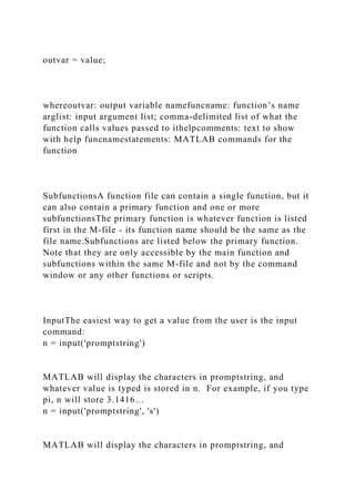
plotting commands, MATLAB allows you to label and annotate
your graphs using the title, xlabel, ylabel, and legend
commands.
Plotting Example
t = [0:2:20]’;
g = 9.81; m = 68.1; cd = 0.25;
v = sqrt(g*m/cd) * tanh(sqrt(g*cd/m)*t);
plot(t, v)
Plotting Annotation Example
title('Plot of v versus t')
xlabel('Values of t')
ylabel('Values of v')
grid
Plotting OptionsWhen plotting data, MATLAB can use several
different colors, point styles, and line styles. These are

specified at the end of the plot command using plot specifiers as
found in Table 2.2.The default case for a single data set is to
create a blue line with no points. If a line style is specified
with no point style, no point will be drawn at the individual
points; similarly, if a point style is specified with no point
style, no line will be drawn.Examples of plot specifiers:‘ro:’ -
red dotted line with circles at the points‘gd’ - green diamonds at
the points with no line‘m--’ - magenta dashed line with no point
symbols
Other Plotting Commands
hold on and hold off
hold on tells MATLAB to keep the current data plotted and add
the results of any further plot commands to the graph. This
continues until the hold off command, which tells MATLAB to
clear the graph and start over if another plotting command is
given. hold on should be used after the first plot in a series is
made.
subplot(m, n, p)
subplot splits the figure window into an mxn array of small axes
and makes the pth one active. Note - the first subplot is at the
top left, then the numbering continues across the row. This is
different from how elements are numbered within a matrix!
Chapter3rev1.ppt
Part 1
Chapter 3

Programming with MATLAB
Chapter ObjectivesLearning how to create well-documented M-
files in the edit window and invoke them from the command
window.Understanding how script and function files
differ.Understanding how to incorporate help comments in
functions.Knowing how to set up M-files so that they
interactively prompt users for information and display results in
the command window.Understanding the role of subfunctions
and how the are accessed.Knowing how to create and retrieve
data files.
Objectives (cont)Learning how to write clear and well-
documented M-files by employing structured programming
constructs to implement logic and repetition.Recognizing the
difference between if...elseif and switch constructs.Recognizing
the difference between for...end and while
structures.Understanding what is meant by vectorization and
why it is beneficial.Knowing how to animate MATLAB
plots.Understanding how anonymous functions can be employed
to pass function functions to function M-files.
M-filesWhile commands can be entered directly to the command
window, MATLAB also allows you to put commands in text
files called M-files. M-files are so named because the files are

stored with a .m extension.There are two main kinds of M-file
Script files
Function files
Script FilesA script file is merely a set of MATLAB commands
that are saved on a file - when MATLAB runs a script file, it is
as if you typed the characters stored in the file on the command
window.Scripts can be executed either by typing their name
(without the .m) in the command window, by selecting the
Debug, Run (or Save and Run) command in the editing window,
or by hitting the F5 key while in the editing window. Note that
the latter two options will save any edits you have made, while
the former will run the file as it exists on the drive.
Function FilesFunction files serve an entirely different purpose
from script files. Function files can accept input arguments
from and return outputs to the command window, but variables
created and manipulated within the function do not impact the
command window.
Function File SyntaxThe general syntax for a function is:
function outvar = funcname(arglist)
% helpcomments
statements

outvar = value;
whereoutvar: output variable namefuncname: function’s name
arglist: input argument list; comma-delimited list of what the
function calls values passed to ithelpcomments: text to show
with help funcnamestatements: MATLAB commands for the
function
SubfunctionsA function file can contain a single function, but it
can also contain a primary function and one or more
subfunctionsThe primary function is whatever function is listed
first in the M-file - its function name should be the same as the
file name.Subfunctions are listed below the primary function.
Note that they are only accessible by the main function and
subfunctions within the same M-file and not by the command
window or any other functions or scripts.
InputThe easiest way to get a value from the user is the input
command:
n = input('promptstring')
MATLAB will display the characters in promptstring, and
whatever value is typed is stored in n. For example, if you type
pi, n will store 3.1416…
n = input('promptstring', 's')
MATLAB will display the characters in promptstring, and

whatever characters are typed will be stored as a string in n.
For example, if you type pi, n will store the letters p and i in a
2x1 char array.
OutputThe easiest way to display the value of a matrix is to
type its name, but that will not work in function or script files.
Instead, use the disp command
disp(value)
will show the value on the screen.If value is a string, enclose
it in single quotes.
Formatted OutputFor formatted output, or for output generated
by combining variable values with literal text, use the fprintf
command:
fprintf('format', x, y,...)
where format is a string specifying how you want the value
of the variables x, y, and more to be displayed - including
literal text to be printed along with the values.The values in the
variables are formatted based on format codes.
Format and Control CodesWithin the format string, the
following format codes define how a numerical value is

displayed:
%d - integer format
%e - scientific format with lowercase e
%E - scientific format with uppercase E
%f - decidmal format
%g - the more compact of %e or %fThe following control codes
produce special results within the format string:
n - start a new line
t - tab
- print the characterTo print a ' put a pair of ' in the format
string
Creating and Accessing FilesMATLAB has a built-in file format
that may be used to save and load the values in variables.
save filename var1 var2 ... varn
saves the listed variables into a file named filename.mat. If no

variable is listed, all variables are saved.
load filename var1 var2 ...varn
loads the listed variables from a file named filename.mat. If no
variable is listed, all variables in the file are loaded. Note -
these are not text files!
ASCII Files To create user-readable files, append the flag
-ascii to the end of a save command. This will save the data to
a text file in the same way that disp sends the data to a
screen.Note that in this case, MATLAB does not append
anything to the file name so you may want to add an extension
such as .txt or .dat.To load a rectangular array from a text file,
simply use the load command and the file name. The data will
be stored in a matrix with the same name as the file (but without
any extension).
Structured ProgrammingStructured programming allows
MATLAB to make decisions or selections based on conditions
of the program.Decisions in MATLAB are based on the result of
logical and relational operations and are implemented with if,
if…else, and if…elseif structures.Selections in MATLAB are
based on comparisons with a test expression and are
implemented with switch structures.
Relational OperatorsFrom Table 3.2: Summary of relational
operators in MATLAB:ExampleOperatorRelationshipx ==

0==Equalunit ~= ‘m’~=Not equala < 0<Less thans > t>Greater
than3.9 <= a/3<=Less than or equal tor >= 0>=Greater than or
equal to
Logical Operators
~x (Not): true if x is false (or zero); false otherwise
x & y (And): true if both x and y are true (or non-zero)
x | y (Or): true if either x or y are true (or non-zero)
Order of OperationsPriority can be set using parentheses. After
that, Mathematical expressions are highest priority, followed by
relational operators, followed by logical operators. All things
being equal, expressions are performed from left to right.Not is
the highest priority logical operator, followed by And and
finally OrGenerally, do not combine two relational operators!
If x=5, 3<x<4 should be false (mathematically), but it is
calculated as an expression in MATLAB as:
3<5<4, which leads to true<4 at which point true is converted to
1, and 1<4 is true!Use (3<x)&(x<4) to properly evaluate.
DecisionsDecisions are made in MATLAB using if structures,
which may also include several elseif branches and possibly a
catch-all else branch.Deciding which branch runs is based on
the result of conditions which are either true or false.
If an if tree hits a true condition, that branch (and that branch
only) runs, then the tree terminates.

If an if tree gets to an else statement without running any prior
branch, that branch will run.Note - if the condition is a matrix,
it is considered true if and only if all entries are true (or non-
zero).
SelectionsSelections are made in MATLAB using switch
structures, which may also include a catch-all otherwise
choice.Deciding which branch runs is based on comparing the
value in some test expression with values attached to different
cases.
If the test expression matches the value attached to a case, that
case’s branch will run.
If no cases match and there is an otherwise statement, that
branch will run.
LoopsAnother programming structure involves loops, where the
same lines of code are run several times. There are two types of
loop:
A for loop ends after a specified number of repetitions
established by the number of columns given to an index
variable.
A while loop ends on the basis of a logical condition.
for LoopsOne common way to use a for…end structure is:
for index = start:step:finish
statements

end
where the index variable takes on successive values in the
vector created using the : operator.
VectorizationSometimes, it is more efficient to have MATLAB
perform calculations on an entire array rather than processing
an array element by element. This can be done through
vectorization.for loopVectorizationi = 0; for t = 0:0.02:50 i = i
+ 1; y(i) = cos(t); endt = 0:0.02:50;
y = cos(t);
while LoopsA while loop is fundamentally different from a for
loop since while loops can run an indeterminate number of
times. The general syntax is
while condition
statements
end
where the condition is a logical expression. If the condition is
true, the statements will run and when that is finished, the loop
will again check on the condition.Note - though the condition
may become false as the statements are running, the only time
it matters is after all the statements have run.

Early TerminationSometimes it will be useful to break out of a
for or while loop early - this can be done using a break
statement, generally in conjunction with an if
structure.Example:
x = 24
while (1)
x = x - 5
if x < 0, break, end
end
will produce x values of 24, 19, 14, 9, 4, and -1, then stop.
AnimationTwo ways to animate plots in MATLAB:
Using looping with simple plotting functions
This approach merely replots the graph over and over again.
Important to use the axis command so that the plots scales are
fixed.
Using special function: getframe and movie
This allows you to capture a sequence of plots (getframe) and
then play them back (movie).

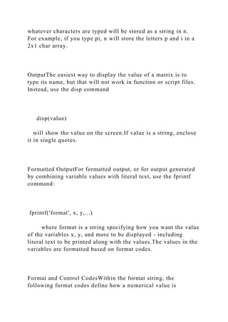
ExampleThe (x, y) coordinates of a projectile can be generated
as a function of time, t,with the following parametric equations
- 0.5 gt2
where v0 = initial velocity (m/s)
q0 = initial angle (radians)
g = gravitational constant (= 9.81 m/s2)
ScriptThe following code illustrates both approaches:
clc,clf,clear
g=9.81; theta0=45*pi/180; v0=5;
t(1)=0;x=0;y=0;
plot(x,y,'o','MarkerFaceColor','b','MarkerSize',8)
axis([0 3 0 0.8])
M(1)=getframe;
dt=1/128;
for j = 2:1000
t(j)=t(j-1)+dt;
x=v0*cos(theta0)*t(j);
y=v0*sin(theta0)*t(j)-0.5*g*t(j)^2;
plot(x,y,'o','MarkerFaceColor','b','MarkerSize',8)
axis([0 3 0 0.8])
M(j)=getframe;
if y<=0, break, end
end
pause
movie(M,1)

Result
Nesting and IndentationStructures can be placed within other
structures. For example, the statements portion of a for loop
can be comprised of an if...elseif...else structure.For clarity of
reading, the statements of a structure are generally indented to
show which lines of controlled are under the control of which
structure.
Anonymous & Inline FunctionsAnonymous functions are simple
one-line functions created without the need for an M-file
fhandle = @(arg1, arg2, ...) expressionInline functions are
essentially the same as anonymous functions, but with a
different syntax:
fhandle = inline('expression', 'arg1', 'arg2',...)Anonymous
functions can access the values of variables in the workspace
upon creation, while inlines cannot.
Function FunctionsFunction functions are functions that operate
on other functions which are passed to it as input arguments.
The input argument may be the handle of an anonymous or
inline function, the name of a built-in function, or the name of a
M-file function.Using function functions will allow for more
dynamic programming.

Chapter4rev1.ppt
Part 1
Chapter 4
Roundoff and
Truncation Errors
Chapter ObjectivesUnderstanding the distinction between
accuracy and precision.Learning how to quantify error.Learning
how error estimates can be used to decide when to terminate an
iterative calculation.Understanding how roundoff errors occur
because digital computers have a limited ability to represent
numbers.Understanding why floating-point numbers have limits
on their range and precision.
Objectives (cont)Recognizing that truncation errors occur when

exact mathematical formulations are represented by
approximations.Knowing how to use the Taylor series to
estimate truncation errors.Understanding how to write forward,
backward, and centered finite-difference approximations of the
first and second derivatives.Recognizing that efforts to
minimize truncation errors can sometimes increase roundoff
errors.
Accuracy and PrecisionAccuracy refers to how closely a
computed or measured value agrees with the true value, while
precision refers to how closely individual computed or
measured values agree with each other.
inaccurate and imprecise
accurate and imprecise
inaccurate and precise
accurate and precise
Error DefinitionsTrue error (Et): the difference between the true
value and the approximation.Absolute error (|Et|): the absolute
difference between the true value and the approximation.True
fractional relative error: the true error divided by the true
expressed as a percentage.

Error Definitions (cont)The previous definitions of error relied
on knowing a true value. If that is not the case, approximations
can be made to the error.The approximate percent relative error
can be given as the approximate error divided by the
approximation, expressed as a percentage - though this presents
the challenge of finding the approximate error!For iterative
processes, the error can be approximated as the difference in
values between sucessive iterations.
Using Error EstimatesOften, when performing calculations, we
may not be concerned with the sign of the error but are
interested in whether the absolute value of the percent relative
referred to as a stopping criterion.
Roundoff ErrorsRoundoff errors arise because digital computers
cannot represent some quantities exactly. There are two major
facets of roundoff errors involved in numerical
calculations:Digital computers have size and precision limits on
their ability to represent numbers.Certain numerical
manipulations are highly sensitive to roundoff errors.
Computer Number RepresentationBy default, MATLAB has
adopted the IEEE double-precision format in which eight bytes
(64 bits) are used to represent floating-point numbers:
n = ±(1+f) x 2eThe sign is determined by a sign bitThe mantissa
f is determined by a 52-bit binary numberThe exponent e is

determined by an 11-bit binary number, from which 1023 is
subtracted to get e
Floating Point RangesValues of -1023 and +1024 for e are
reserved for special meanings, so the exponent range is -1022 to
1023.The largest possible number MATLAB can store has
f of all 1’s, giving a significand of 2 - 2-52, or approximately 2
e of 111111111102, giving an exponent of 2046 - 1023 = 1023
10308The smallest
possible number MATLAB can store with full precision has
f of all 0’s, giving a significand of 1
e of 000000000012, giving an exponent of 1-1023 = -1022
This yields 2- -308
Floating Point PrecisionThe 52 bits for the mantissa f
correspond to about 15 to 16 base-10 digits. The machine
epsilon - the maximum relative error between a number and
MATLAB’s representation of that number, is thus
2- -16
Roundoff Errors with
Arithmetic ManipulationsRoundoff error can happen in several
circumstances other than just storing numbers - for
example:Large computations - if a process performs a large
number of computations, roundoff errors may build up to
become significantAdding a Large and a Small Number - Since

the small number’s mantissa is shifted to the right to be the
same scale as the large number, digits are lostSmearing -
Smearing occurs whenever the individual terms in a summation
are larger than the summation itself. (x + 10-20) - x = 10-20
mathematically, but
x = 1; (x + 10-20) - x gives a 0 in MATLAB!
Truncation ErrorsTruncation errors are those that result from
using an approximation in place of an exact mathematical
procedure.Example 1: approximation to a derivative using a
finite-difference equation:
Example 2: The Taylor Series
The Taylor Theorem and SeriesThe Taylor theorem states that
any smooth function can be approximated as a polynomial.The
Taylor series provides a means to express this idea
mathematically.
The Taylor Series
Truncation ErrorIn general, the nth order Taylor series

expansion will be exact for an nth order polynomial.In other
cases, the remainder term Rn is of the order of hn+1, meaning:
The more terms are used, the smaller the error, and
The smaller the spacing, the smaller the error for a given
number of terms.
Numerical DifferentiationThe first order Taylor series can be
used to calculate approximations to derivatives:
Given:
Then:
This is termed a “forward” difference because it utilizes data at
i and i+1 to estimate the derivative.
Differentiation (cont)There are also backward and centered
difference approximations, depending on the points
used:Forward:
Backward:
Centered:
Total Numerical ErrorThe total numerical error is the
summation of the truncation and roundoff errors.The truncation
error generally increases as the step size increases, while the

roundoff error decreases as the step size increases - this leads to
a point of diminishing returns for step size.
Other ErrorsBlunders - errors caused by malfunctions of the
computer or human imperfection.Model errors - errors resulting
from incomplete mathematical models.Data uncertainty - errors
resulting from the accuracy and/or precision of the data.
dv
dt
@
D
v
D
t
=
v
(
t
i
+
1
)
-
v
(
t
i

)
t
i
+
1
-
t
i
f
x
i
+
1
(
)
=
f
x
i
(
)
+
f
'
x
i
(
)
h
+
f
'
'
x

i
(
)
2
!
h
2
+
f
(
3
)
x
i
(
)
3
!
h
3
+
L
+
f
(
n
)
x
i
(
)
n
!
h
n
+

R
n
f
'
(
x
i
)
=
f
(
x
i
)
-
f
(
x
i
-
1
)
h
+
O
(
h
)
f
(
x
i
+
1

)
=
f
(
x
i
)
+
f
'
(
x
i
)
h
+
O
(
h
2
)
f
'
(
x
i
)
=
f
(
x
i
+
1
)

-
f
(
x
i
)
h
+
O
(
h
)
f
'
(
x
i
)
=
f
(
x
i
+
1
)
-
f
(
x
i
-
1
)
2

h
+
O
(
h
2
)
Chapter5rev1.ppt
Part 2
Chapter 5
Roots: Bracketing Methods
University
Chapter ObjectivesUnderstanding what roots problems are and
where they occur in engineering and science.Knowing how to
determine a root graphically.Understanding the incremental
search method and its shortcomings.Knowing how to solve a
roots problem with the bisection method.Knowing how to
estimate the error of bisection and why it differs from error
estimates for other types of root location
algorithms.Understanding false position and how it differs from
bisection.

Roots“Roots” problems occur when some function f can be
written in terms of one or more dependent variables x, where
the solutions to f(x)=0 yields the solution to the problem.These
problems often occur when a design problem presents an
implicit equation for a required parameter.
Graphical MethodsA simple method for obtaining the estimate
of the root of the equation f(x)=0 is to make a plot of the
function and observe where it crosses the x-axis.Graphing the
function can also indicate where roots may be and where some
root-finding methods may fail:
Same sign, no roots
Different sign, one root
Same sign, two roots
Different sign, three roots
Bracketing MethodsBracketing methods are based on making
two initial guesses that “bracket” the root - that is, are on either
side of the root.Brackets are formed by finding two guesses xl
and xu where the sign of the function changes; that is, where
f(xl ) f(xu ) < 0The incremental search method tests the value of
the function at evenly spaced intervals and finds brackets by
identifying function sign changes between neighboring points.
Incremental Search HazardsIf the spacing between the points of
an incremental search are too far apart, brackets may be missed
due to capturing an even number of roots within two
points.Incremental searches cannot find brackets containing
even-multiplicity roots regardless of spacing.

BisectionThe bisection method is a variation of the incremental
search method in which the interval is always divided in half.If
a function changes sign over an interval, the function value at
the midpoint is evaluated.The location of the root is then
determined as lying within the subinterval where the sign
change occurs.The absolute error is reduced by a factor of 2 for
each iteration.
Programming Bisection
Bisection ErrorThe absolute error of the bisection method is
solely dependent on the absolute error at the start of the process
(the space between the two guesses) and the number of
iterations:
The required number of iterations to obtain a particular absolute
error can be calculated based on the initial guesses:
False PositionThe false position method is another bracketing
method.It determines the next guess not by splitting the bracket
in half but by connecting the endpoints with a straight line and
determining the location of the intercept of the straight line
(xr).The value of xr then replaces whichever of the two initial
guesses yields a function value with the same sign as f(xr).

False Position Illustration
Bisection vs. False PositionBisection does not take into account
the shape of the function; this can be good or bad depending on
the function!Bad:
E
a
n
=
D
x
0
2
n
n
=
log
2
D
x
0
E
a
,
d
æ
è
ç

ö
ø
÷
x
r
=
x
u
-
f
(
x
u
)(
x
l
-
x
u
)
f
(
x
l
)
-
f
(
x
u
)
f
(
x

)
=
x
10
-
1
Chapter6rev1.ppt
Part 2
Chapter 6
Roots: Open Methods
University
Chapter ObjectivesRecognizing the difference between
bracketing and open methods for root location.Understanding
the fixed-point iteration method and how you can evaluate its
convergence characteristics.Knowing how to solve a roots
problem with the Newton-Raphson method and appreciating the
concept of quadratic convergence.Knowing how to implement
both the secant and the modified secant methods.Knowing how
to use MATLAB’s fzero function to estimate roots.Learning
how to manipulate and determine the roots of polynomials with
MATLAB.

Open MethodsOpen methods differ from bracketing methods, in
that open methods require only a single starting value or two
starting values that do not necessarily bracket a root.Open
methods may diverge as the computation progresses, but when
they do converge, they usually do so much faster than
bracketing methods.
Graphical Comparison of Methods
Bracketing method
Diverging open method
Converging open method - note speed!
Simple Fixed-Point IterationRearrange the function f(x)=0 so
that x is on the left-hand side of the equation: x=g(x)Use the
new function g to predict a new value of x - that is,
xi+1=g(xi)The approximate error is given by:
ExampleSolve f(x)=e-x-xRe-write as x=g(x) by isolating x
(example: x=e-x)Start with an initial guess (here, 0)
Continue until some tolerance

-
100.0000100.00011.0000100.000 76.3220.76320.3679171.828
35.1350.46030.6922 46.854 22.0500.62840.5005 38.309
11.7550.533
ConvergenceConvergence of the simple fixed-point iteration
method requires that the derivative of g(x) near the root has a
magnitude less than 1.
Convergent, 0≤g’<1
Convergent, -1<g’≤0
Divergent, g’>1
Divergent, g’<-1
Newton-Raphson MethodBased on forming the tangent line to
the f(x) curve at some guess x, then following the tangent line
to where it crosses the x-axis.
Pros and ConsPro: The error of the i+1th iteration is roughly
proportional to the square of the error of the ith iteration - this
is called quadratic convergenceCon: Some functions show slow
or poor convergence
Secant MethodsA potential problem in implementing the
Newton-Raphson method is the evaluation of the derivative -
there are certain functions whose derivatives may be difficult or
inconvenient to evaluate.For these cases, the derivative can be

approximated by a backward finite divided difference:
Secant Methods (cont)Substitution of this approximation for the
derivative to the Newton-Raphson method equation gives:
Note - this method requires two initial estimates of x but does
not require an analytical expression of the derivative.
MATLAB’s fzero FunctionMATLAB’s fzero provides the best
qualities of both bracketing methods and open methods.Using
an initial guess:
x = fzero(function, x0)
[x, fx] = fzero(function, x0)function is a function handle to the
function being evaluatedx0 is the initial guessx is the location
of the rootfx is the function evaluated at that rootUsing an
initial bracket:
x = fzero(function, [x0 x1])
[x, fx] = fzero(function, [x0 x1])As above, except x0 and x1 are
guesses that must bracket a sign change

fzero OptionsOptions may be passed to fzero as a third input
argument - the options are a data structure created by the
optimset commandoptions = optimset(‘par1’, val1, ‘par2’,
val2,…)parn is the name of the parameter to be setvaln is the
value to which to set that parameterThe parameters commonly
used with fzero are:display: when set to ‘iter’ displays a
detailed record of all the iterationstolx: A positive scalar that
sets a termination tolerance on x.
fzero Exampleoptions = optimset(‘display’, ‘iter’);Sets options
to display each iteration of root finding process[x, fx] =
fzero(@(x) x^10-1, 0.5, options)Uses fzero to find roots of
f(x)=x10-1 starting with an initial guess of x=0.5.MATLAB
reports x=1, fx=0 after 35 function counts
PolynomialsMATLAB has a built in program called roots to
determine all the roots of a polynomial - including imaginary
and complex ones.x = roots(c)x is a column vector containing
the rootsc is a row vector containing the polynomial
coefficientsExample:Find the roots of
f(x)=x5-3.5x4+2.75x3+2.125x2-3.875x+1.25x = roots([1 -3.5
2.75 2.125 -3.875 1.25])
Polynomials (cont)MATLAB’s poly function can be used to
determine polynomial coefficients if roots are given:b =
poly([0.5 -1])Finds f(x) where f(x) =0 for x=0.5 and x=-
1MATLAB reports b = [1.000 0.5000 -0.5000]This corresponds
to f(x)=x2+0.5x-0.5MATLAB’s polyval function can evaluate a

polynomial at one or more points:a = [1 -3.5 2.75 2.125 -3.875
1.25];If used as coefficients of a polynomial, this corresponds
to f(x)=x5-3.5x4+2.75x3+2.125x2-3.875x+1.25polyval(a, 1)This
calculates f(1), which MATLAB reports as -0.2500
e
a
=
x
i
+
1
-
x
i
x
i
+
1
100
%
f
'
(
x
i
)
=
f
(
x
i
)

-
0
x
i
-
x
i
+
1
x
i
+
1
=
x
i
-
f
(
x
i
)
f
'
(
x
i
)
f
'
(
x
i
)
@

f
(
x
i
-
1
)
-
f
(
x
i
)
x
i
-
1
-
x
i
x
i
+
1
=
x
i
-
f
(
x
i
)
x
i

-
1
-
x
i
(
)
f
(
x
i
-
1
)
-
f
(
x
i
)
Chapter7rev1.ppt
Part 2
Chapter 7
Optimization
University

Chapter ObjectivesUnderstanding why and where optimization
occurs in engineering and scientific problem
solving.Recognizing the difference between one-dimensional
and multi-dimensional optimization.Distinguishing between
global and local optima.Knowing how to recast a maximization
problem so that it can be solved with a minimizing
algorithm.Being able to define the golden ratio and understand
why it makes one-dimensional optimization efficient.
Objectives (cont)Locating the optimum of a single-variable
function with the golden-section search.Locating the optimum
of a single-variable function with parabolic
interpolation.Knowing how to apply the fminbnd function to
determine the minimum of a one-dimensional function.Being
able to develop MATLAB contours and surface plots to
visualize two-dimensional functions.Knowing how to apply the
fminsearch function to determine the minimum of a
multidimensional function.
OptimizationOptimization is the process of creating something
that is as effective as possible.From a mathematical perspective,
optimization deals with finding the maxima and minima of a
function that depends on one or more variables.
Multidimensional OptimizationOne-dimensional problems
involve functions that depend on a single dependent variable -
for example, f(x).Multidimensional problems involve functions
that depend on two or more dependent variables - for example,

f(x,y)
Global vs. LocalA global optimum represents the very best
solution while a local optimum is better than its immediate
neighbors. Cases that include local optima are called
multimodal.Generally desire to find the global optimum.
Golden-Section SearchSearch algorithm for finding a minimum
on an interval [xl xu] with a single minimum (unimodal
of two interior points x1 and x2; by using the golden ratio, one
of the interior points can be re-used in the next iteration.
Golden-Section Search (cont)
If f(x1)<f(x2), x2 becomes the new lower limit and x1 becomes
the new x2 (as in figure).If f(x2)<f(x1), x1 becomes the new
upper limit and x2 becomes the new x1.In either case, only one
new interior point is needed and the function is only evaluated
one more time.
Code for Golden-Section Search
Parabolic InterpolationAnother algorithm uses parabolic

interpolation of three points to estimate optimum location.The
location of the maximum/minimum of a parabola defined as the
interpolation of three points (x1, x2, and x3) is:
The new point x4 and the two
surrounding it (either x1 and x2
or x2 and x3) are used for the
next iteration of the algorithm.
fminbnd FunctionMATLAB has a built-in function, fminbnd,
which combines the golden-section search and the parabolic
interpolation.[xmin, fval] = fminbnd(function, x1, x2)Options
may be passed through a fourth argument using optimset,
similar to fzero.
Multidimensional VisualizationFunctions of two-dimensions
may be visualized using contour or surface/mesh plots.
fminsearch FunctionMATLAB has a built-in function,
fminsearch, that can be used to determine the minimum of a
multidimensional function.[xmin, fval] = fminsearch(function,
x0)xmin in this case will be a row vector containing the location

of the minimum, while x0 is an initial guess. Note that x0 must
contain as many entries as the function expects of it.The
function must be written in terms of a single variable, where
different dimensions are represented by different indices of that
variable.
fminsearch FunctionTo minimize
f(x,y)=2+x-y+2x2+2xy+y2
rewrite as
f(x1, x2)=2+x1-x2+2(x1)2+2x1x2+(x2)2[email protected](x)
2+x(1)-x(2)+2*x(1)^2+2*x(1)*x(2)+x(2)^2
[x, fval] = fminsearch(f, [-0.5, 0.5])Note that x0 has two entries
- f is expecting it to contain two values.MATLAB reports the
minimum value is 0.7500 at a location of [-1.000 1.5000]
d
=
(
f
-
1
)(
x
u
-

x
l
)
x
1
=
x
l
+
d
x
2
=
x
u
-
d
x
4
=
x
2
-
1
2
x
2
-
x
1
(
)
2
f
x

2
(
)
-
f
x
3
(
)
[
]
-
x
2
-
x
3
(
)
2
f
x
2
(
)
-
f
x
1
(
)
[
]
x
2
-

x
1
(
)
f
x
2
(
)
-
f
x
3
(
)
[
]
-
x
2
-
x
3
(
)
f
x
2
(
)
-
f
x
1
(
)

[
]
Chapter8rev1.ppt
Part 3
Chapter 8
Linear Algebraic Equations and Matrices
University
Chapter ObjectivesUnderstanding matrix notation.Being able to
identify the following types of matrices: identify, diagonal,
symmetric, triangular, and tridiagonal.Knowing how to perform
matrix multiplication and being able to assess when it is
feasible.Knowing how to represent a system of linear equations
in matrix form.Knowing how to solve linear algebraic equations
with left division and matrix inversion in MATLAB.
OverviewA matrix consists of a rectangular array of elements
represented by a single symbol (example: [A]).An individual
entry of a matrix is an element (example: a23)

Overview (cont)A horizontal set of elements is called a row and
a vertical set of elements is called a column.The first subscript
of an element indicates the row while the second indicates the
column.The size of a matrix is given as m rows by n columns,
or simply m by n (or m x n).1 x n matrices are row vectors.m x
1 matrices are column vectors.
Special MatricesMatrices where m=n are called square
matrices.There are a number of special forms of square
matrices:
Matrix OperationsTwo matrices are considered equal if and only
if every element in the first matrix is equal to every
corresponding element in the second. This means the two
matrices must be the same size.Matrix addition and subtraction
are performed by adding or subtracting the corresponding
elements. This requires that the two matrices be the same
size.Scalar matrix multiplication is performed by multiplying
each element by the same scalar.
Matrix MultiplicationThe elements in the matrix [C] that results
from multiplying matrices [A] and [B] are calculated using:
Matrix Inverse and TransposeThe inverse of a square,
nonsingular matrix [A] is that matrix which, when multiplied by
[A], yields the identity matrix.[A][A]-1=[A]-1[A]=[I] The

transpose of a matrix involves transforming its rows into
columns and its columns into rows.(aij)T=aji
Representing Linear AlgebraMatrices provide a concise notation
for representing and solving simultaneous linear equations:
Solving With MATLABMATLAB provides two direct ways to
solve systems of linear algebraic equations [A]{x}={b}:Left-
division
x = AbMatrix inversion
x = inv(A)*bThe matrix inverse is less efficient than left-
division and also only works for square, non-singular systems.
Symmetric
A
[
]
=
5
1
2
1
3

7
2
7
8
é
ë
ê
ê
ê
ù
û
ú
ú
ú
Diagonal
A
[
]
=
a
11
a
22
a
33
é
ë
ê
ê
ê
ù
û
ú
ú
ú
Identity

A
[
]
=
1
1
1
é
ë
ê
ê
ê
ù
û
ú
ú
ú
Upper Triangular
A
[
]
=
a
11
a
12
a
13
a
22
a
23
a
33
é
ë

ê
ê
ê
ù
û
ú
ú
ú
Lower Triangular
A
[
]
=
a
11
a
21
a
22
a
31
a
32
a
33
é
ë
ê
ê
ê
ù
û
ú
ú
ú
Banded

A
[
]
=
a
11
a
12
a
21
a
22
a
23
a
32
a
33
a
34
a
43
a
44
é
ë
ê
ê
ê
ê
ù
û
ú
ú
ú
ú

c
ij
=
a
ik
b
kj
k
=
1
n
å
a
11
x
1
+
a
12
x
2
+
a
13
x
3
=
b
1
a
21
x
1
+

a
22
x
2
+
a
23
x
3
=
b
2
a
31
x
1
+
a
32
x
2
+
a
33
x
3
=
b
3
[
A
]{
x
}
=

{
b
}
a
11
a
12
a
13
a
21
a
22
a
23
a
31
a
32
a
33
é
ë
ê
ê
ê
ù
û
ú
ú
ú
x
1
x
2

x
3
ì
í
ï
î
ï
ü
ý
ï
þ
ï
=
b
1
b
2
b
3
ì
í
ï
î
ï
ü
ý
ï
þ
ï
Chapter9rev1.ppt
Part 3

Chapter 9
Gauss Elimination
University
Chapter ObjectivesKnowing how to solve small sets of linear
equations with the graphical method and Cramer’s
rule.Understanding how to implement forward elimination and
back substitution as in Gauss elimination.Understanding how to
count flops to evaluate the efficiency of an
algorithm.Understanding the concepts of singularity and ill-
condition.Understanding how partial pivoting is implemented
and how it differs from complete pivoting.Recognizing how the
banded structure of a tridiagonal system can be exploited to
obtain extremely efficient solutions.
Graphical MethodFor small sets of simultaneous equations,
graphing them and determining the location of the intercept
provides a solution.
Graphical Method (cont)Graphing the equations can also show
systems where:
No solution exists
Infinite solutions exist
System is ill-conditioned

DeterminantsThe determinant D=|A| of a matrix is formed from
the coefficients of [A].Determinants for small matrices are:
Determinants for matrices larger than 3 x 3 can be very
complicated.
Cramer’s RuleCramer’s Rule states that each unknown in a
system of linear algebraic equations may be expressed as a
fraction of two determinants with denominator D and with the
numerator obtained from D by replacing the column of
coefficients of the unknown in question by the constants b1, b2,
…, bn.
Cramer’s Rule ExampleFind x2 in the following system of
equations:
Find the determinant D
Find determinant D2 by replacing D’s second column with b
Divide

Naïve Gauss EliminationFor larger systems, Cramer’s Rule can
become unwieldy.Instead, a sequential process of removing
unknowns from equations using forward elimination followed
by back substitution may be used - this is Gauss
elimination.“Naïve” Gauss elimination simply means the
process does not check for potential problems resulting from
division by zero.
Naïve Gauss Elimination (cont)Forward eliminationStarting
with the first row, add or subtract multiples of that row to
eliminate the first coefficient from the second row and
beyond.Continue this process with the second row to remove the
second coefficient from the third row and beyond.Stop when an
upper triangular matrix remains.Back substitutionStarting with
the last row, solve for the unknown, then substitute that value
into the next highest row.Because of the upper-triangular nature
of the matrix, each row will contain only one more unknown.
Naïve Gauss Elimination Program
Gauss Program EfficiencyThe execution of Gauss elimination
depends on the amount of floating-point operations (or flops).
The flop count for an n x n system is:

Conclusions:As the system gets larger, the computation time
increases greatly.Most of the effort is incurred in the
elimination step.
PivotingProblems arise with naïve Gauss elimination if a
coefficient along the diagonal is 0 (problem: division by 0) or
close to 0 (problem: round-off error)One way to combat these
issues is to determine the coefficient with the largest absolute
value in the column below the pivot element. The rows can
then be switched so that the largest element is the pivot
element. This is called partial pivoting.If the rows to the right
of the pivot element are also checked and columns switched,
this is called complete pivoting.
Partial Pivoting Program
Tridiagonal SystemsA tridiagonal system is a banded system
with a bandwidth of 3:
Tridiagonal systems can be solved using the same method as
Gauss elimination, but with much less effort because most of
the matrix elements are already 0.

Tridiagonal System Solver
x
2
=
D
2
D
=
0
.
0649
-
0
.
0022
=
-
29
.
5
0
.
3
x
1
+
0
.
52

x
2
+
x
3
=
-
0
.
01
0
.
5
x
1
+
x
2
+
1
.
9
x
3
=
0
.
67
0
.
1
x
1
+
0
.

3
x
2
+
0
.
5
x
3
=
-
0
.
44
D
=
0
.
3
0
.
52
1
0
.
5
1
1
.
9
0
.
1
0
.

3
0
.
5
=
0
.
3
1
1
.
9
0
.
3
0
.
5
-
0
.
52
0
.
5
1
.
9
0
.
1
0
.
5
+
1

0
.
5
1
0
.
1
0
.
4
=
-
0
.
0022
1
´
1
a
11
=
a
11
2
´
2
a
11
a
12
a
21
a
22
=

a
11
a
22
-
a
12
a
21
3
´
3
a
11
a
12
a
13
a
21
a
22
a
23
a
31
a
32
a
33
=
a
11
a
22
a

23
a
32
a
33
-
a
12
a
21
a
23
a
31
a
33
+
a
13
a
21
a
22
a
31
a
32
D
2
=
0
.
3
-
0

.
01
1
0
.
5
0
.
67
1
.
9
0
.
1
-
0
.
44
0
.
5
=
0
.
3
0
.
67
1
.
9
-
0
.
44

0
.
5
-
0
.
01
0
.
5
1
.
9
0
.
1
0
.
5
+
1
0
.
5
0
.
67
0
.
1
-
0
.
44
=
0

.
0649
Forward
Elimination
2
n
3
3
+
O
n
2
(
)
Back
Substitution
n
2
+
O
n
(
)
Total
2
n
3
3
+
O
n
2
(
)

f
1
g
1
e
2
f
2
g
2
e
3
f
3
g
3
×
×
×
×
×
×
×
×
×
e
n
-
1
f
n
-
1
g
n
-

1
e
n
f
n
é
ë
ê
ê
ê
ê
ê
ê
ê
ê
ù
û
ú
ú
ú
ú
ú
ú
ú
ú
x
1
x
2
x
3
×
×
×
x
n

-
1
x
n
ì
í
ï
ï
ï
î
ï
ï
ï
ü
ý
ï
ï
ï
þ
ï
ï
ï
=
r
1
r
2
r
3
×
×
×
r
n
-
1

r
n
ì
í
ï
ï
ï
î
ï
ï
ï
ü
ý
ï
ï
ï
þ
ï
ï
ï
Chapter10rev1.ppt
Part 3
Chapter 10
LU Factorization
University

Chapter ObjectivesUnderstanding that LU factorization involves
decomposing the coefficient matrix into two triangular matrices
that can then be used to efficiently evaluate different right-
hand-side vectors.Knowing how to express Gauss elimination as
an LU factorization.Given an LU factorization, knowing how to
evaluate multiple right-hand-side vectors.Recognizing that
Cholesky’s method provides an efficient way to decompose a
symmetric matrix and that the resulting triangular matrix and its
transpose can be used to evaluate right-hand-side vectors
efficiently.Understanding in general terms what happens when
MATLAB’s backslash operator is used to solve linear systems.
LU FactorizationRecall that the forward-elimination step of
Gauss elimination comprises the bulk of the computational
effort.LU factorization methods separate the time-consuming
elimination of the matrix [A] from the manipulations of the
right-hand-side [b].Once [A] has been factored (or
decomposed), multiple right-hand-side vectors can be evaluated
in an efficient manner.
LU FactorizationLU factorization involves two
steps:Factorization to decompose the [A] matrix into a product
of a lower triangular matrix [L] and an upper triangular matrix
[U]. [L] has 1 for each entry on the diagonal.Substitution to
solve for {x}Gauss elimination can be implemented using LU
factorization
Gauss Elimination as

LU Factorization[A]{x}={b} can be rewritten as [L][U]{x}={b}
using LU factorization.The LU factorization algorithm requires
the same total flops as for Gauss elimination.The main
advantage is once [A] is decomposed, the same [L] and [U] can
be used for multiple {b} vectors.MATLAB’s lu function can be
used to generate the [L] and [U] matrices:
[L, U] = lu(A)
Gauss Elimination as
LU Factorization (cont)To solve [A]{x}={b}, first decompose
[A] to get [L][U]{x}={b}Set up and solve [L]{d}={b}, where
{d} can be found using forward substitution.Set up and solve
[U]{x}={d}, where {x} can be found using backward
substitution.In MATLAB:
[L, U] = lu(A)
d = Lb
x = Ud
Cholesky FactorizationSymmetric systems occur commonly in
both mathematical and engineering/science problem contexts,

and there are special solution techniques available for such
systems.The Cholesky factorization is one of the most popular
of these techniques, and is based on the fact that a symmetric
matrix can be decomposed as [A]= [U]T[U], where T stands for
transpose.The rest of the process is similar to LU decomposition
and Gauss elimination, except only one matrix, [U], needs to be
stored.
MATLABMATLAB can perform a Cholesky factorization with
the built-in chol command:
U = chol(A)MATLAB’s left division operator examines
the system to see which method will most efficiently solve the
problem. This includes trying banded solvers, back and forward
substitutions, Cholesky factorization for symmetric systems. If
these do not work and the system is square, Gauss elimination
with partial pivoting is used.
Chapter11rev1.ppt
Part 3
Chapter 11
Matrix Inverse and Condition
University

Chapter ObjectivesKnowing how to determine the matrix
inverse in an efficient manner based on LU
factorization.Understanding how the matrix inverse can be used
to assess stimulus-response characteristics of engineering
systems.Understanding the meaning of matrix and vector norms
and how they are computed.Knowing how to use norms to
compute the matrix condition number.Understanding how the
magnitude of the condition number can be used to estimate the
precision of solutions of linear algebraic equations.
Matrix InverseRecall that if a matrix [A] is square, there is
another matrix [A]-1, called the inverse of [A], for which
[A][A]-1=[A]-1[A]=[I] The inverse can be computed in a
column by column fashion by generating solutions with unit
vectors as the right-hand-side constants:
Matrix Inverse (cont)Recall that LU factorization can be used to
efficiently evaluate a system for multiple right-hand-side
vectors - thus, it is ideal for evaluating the multiple unit vectors
needed to compute the inverse.
Stimulus-Response Computations

Chapter24rev1.pptPart 6Chapter 24Boundary-Valu.docx

Chapter24rev1.pptPart 6Chapter 24Boundary-Valu.docx

More Related Content

Similar to Chapter24rev1.pptPart 6Chapter 24Boundary-Valu.docx

More from tiffanyd4

Recently uploaded

Chapter24rev1.pptPart 6Chapter 24Boundary-Valu.docx