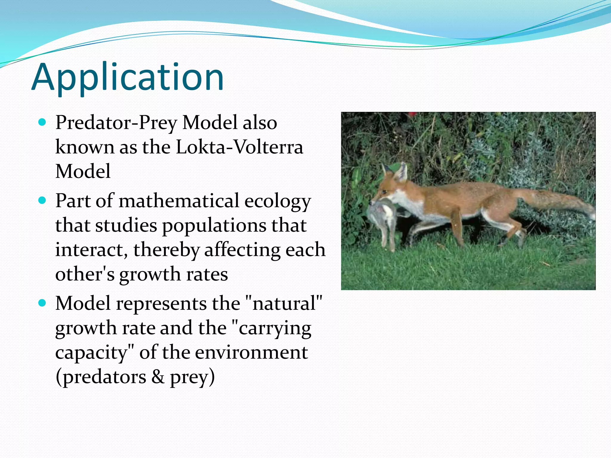
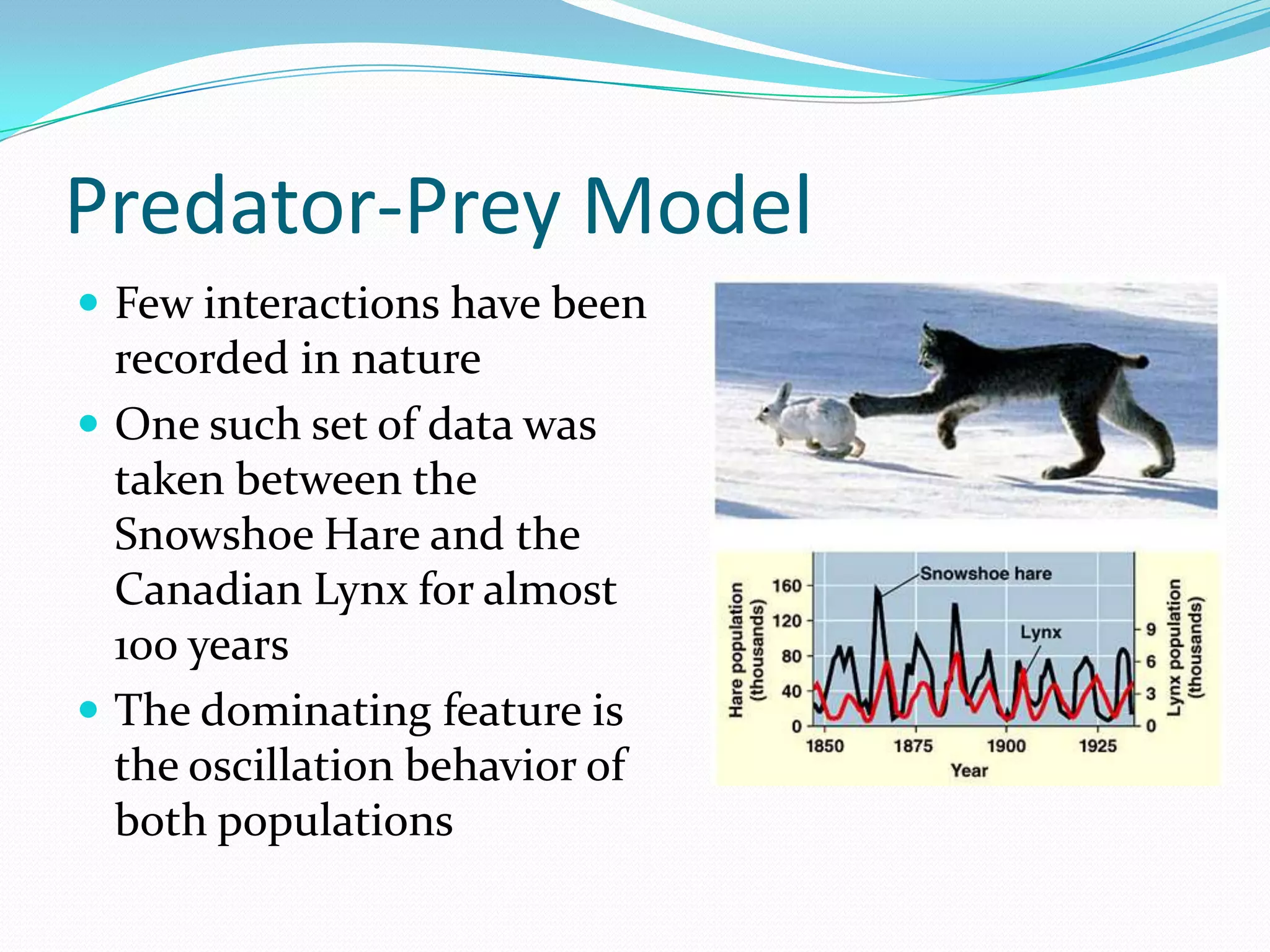
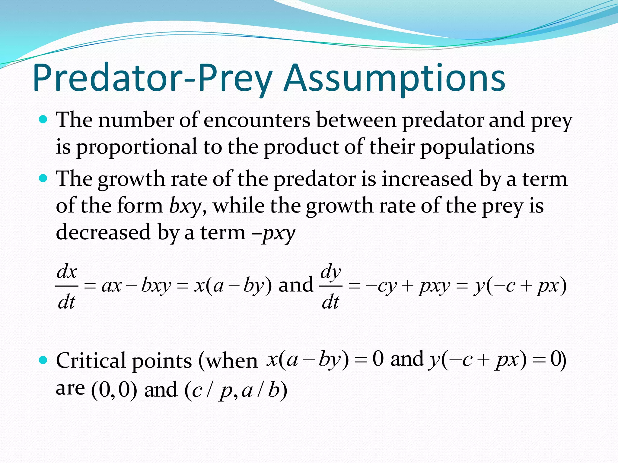
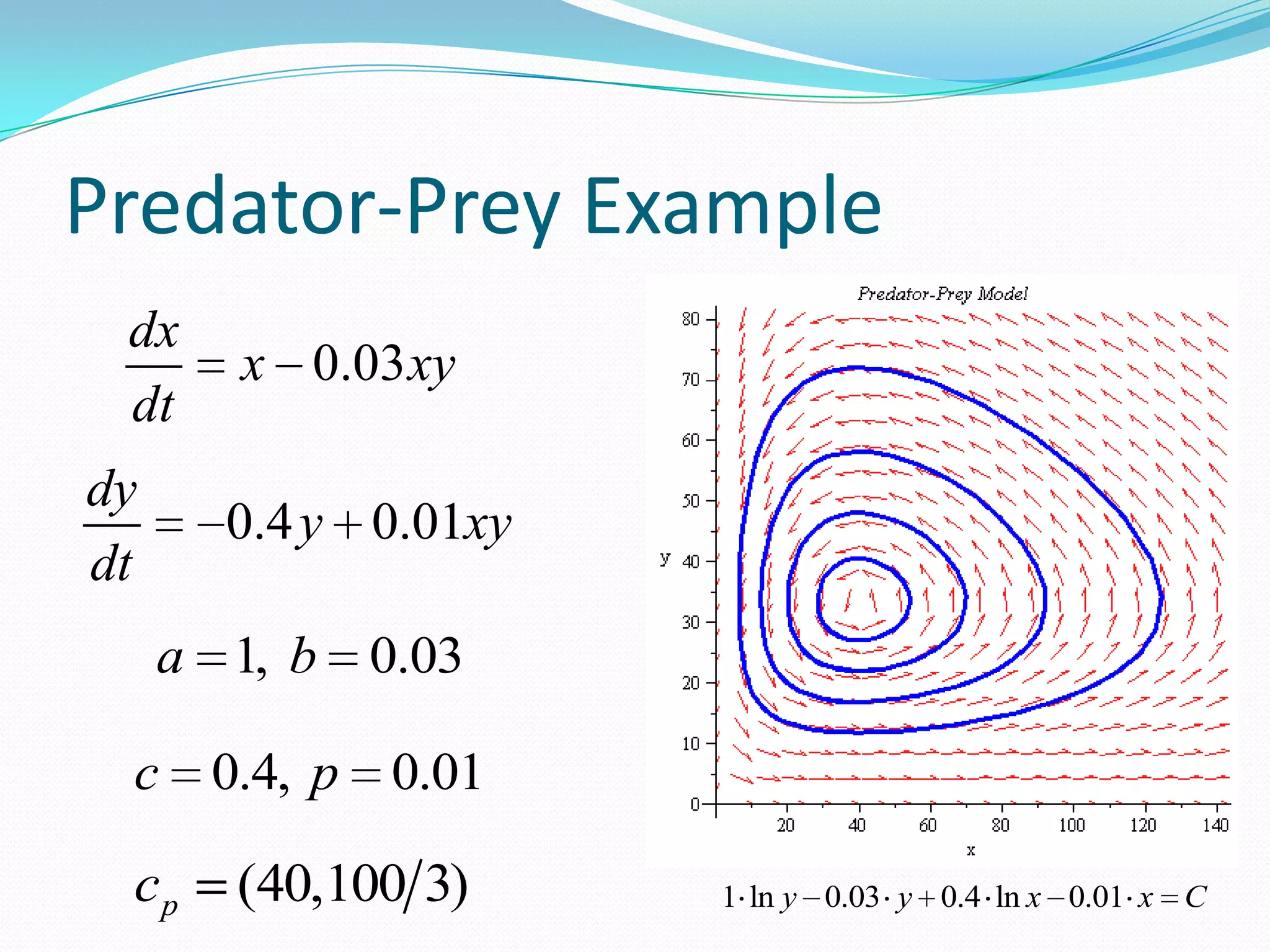
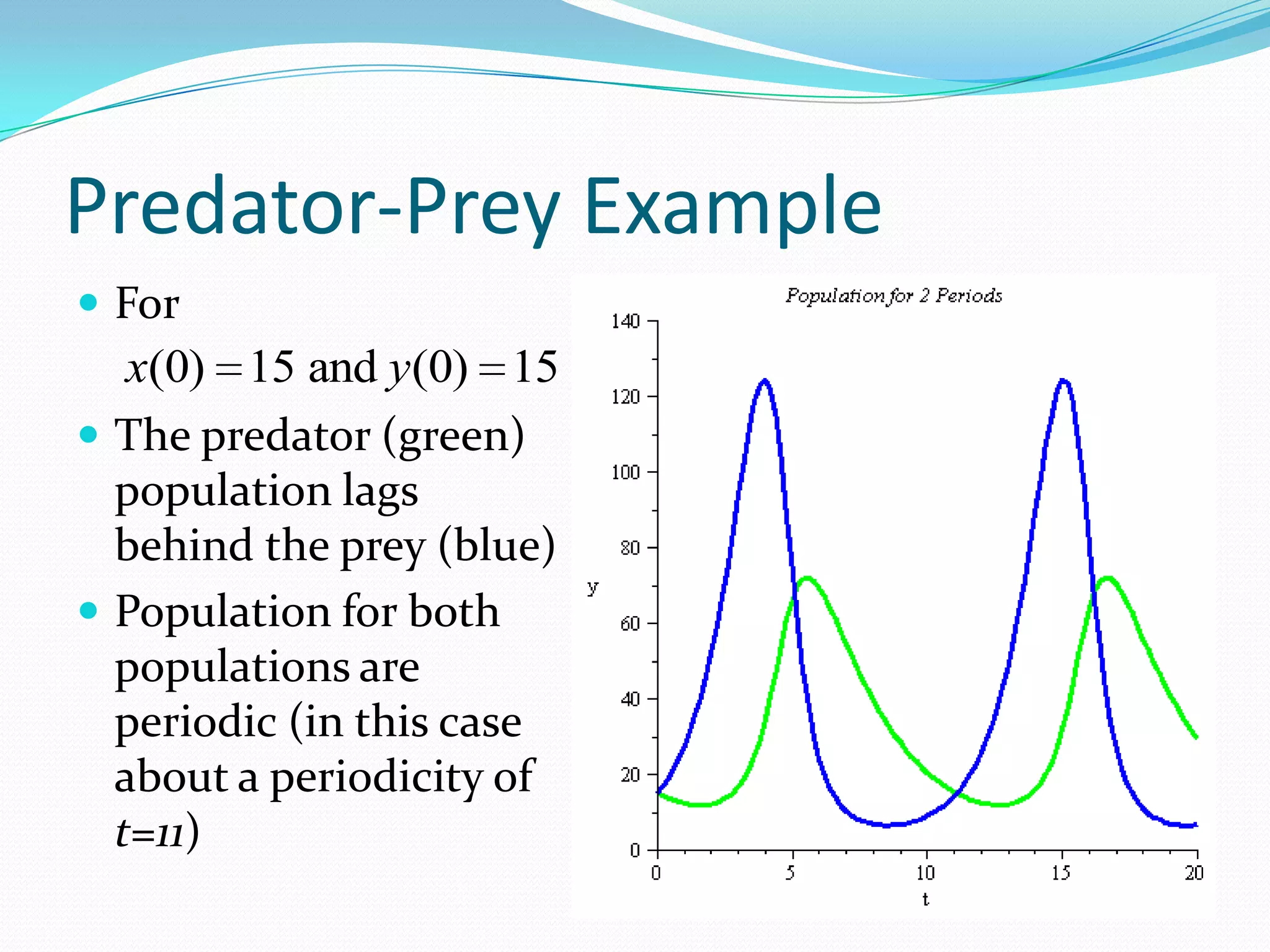
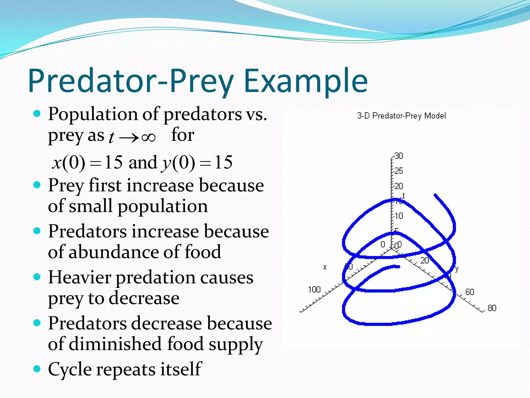
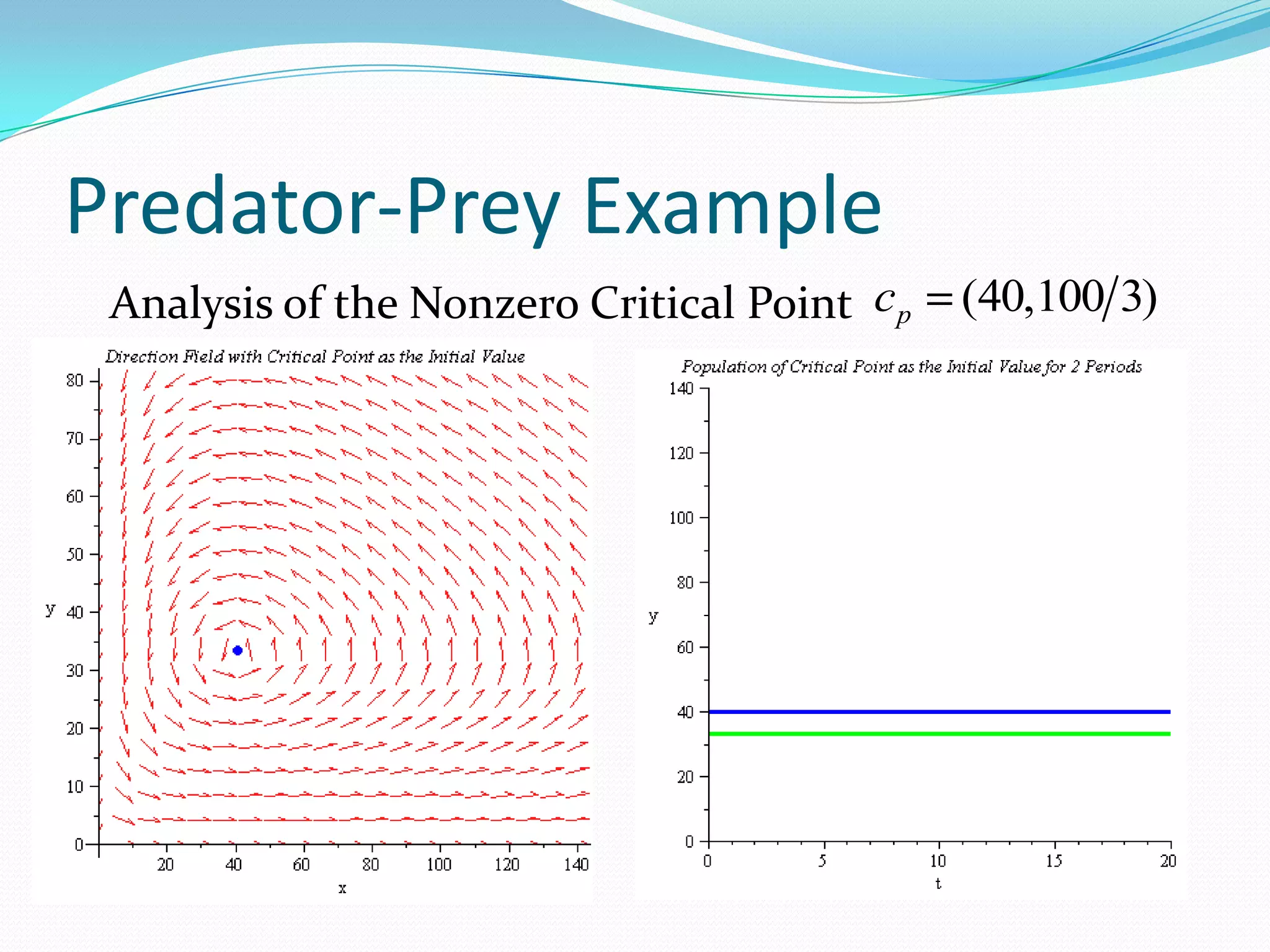
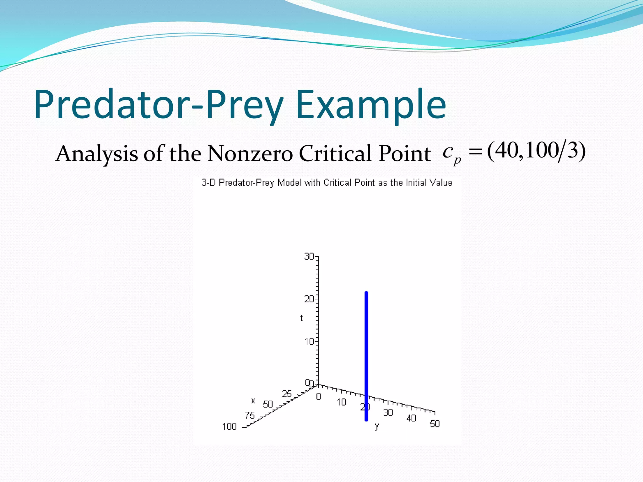
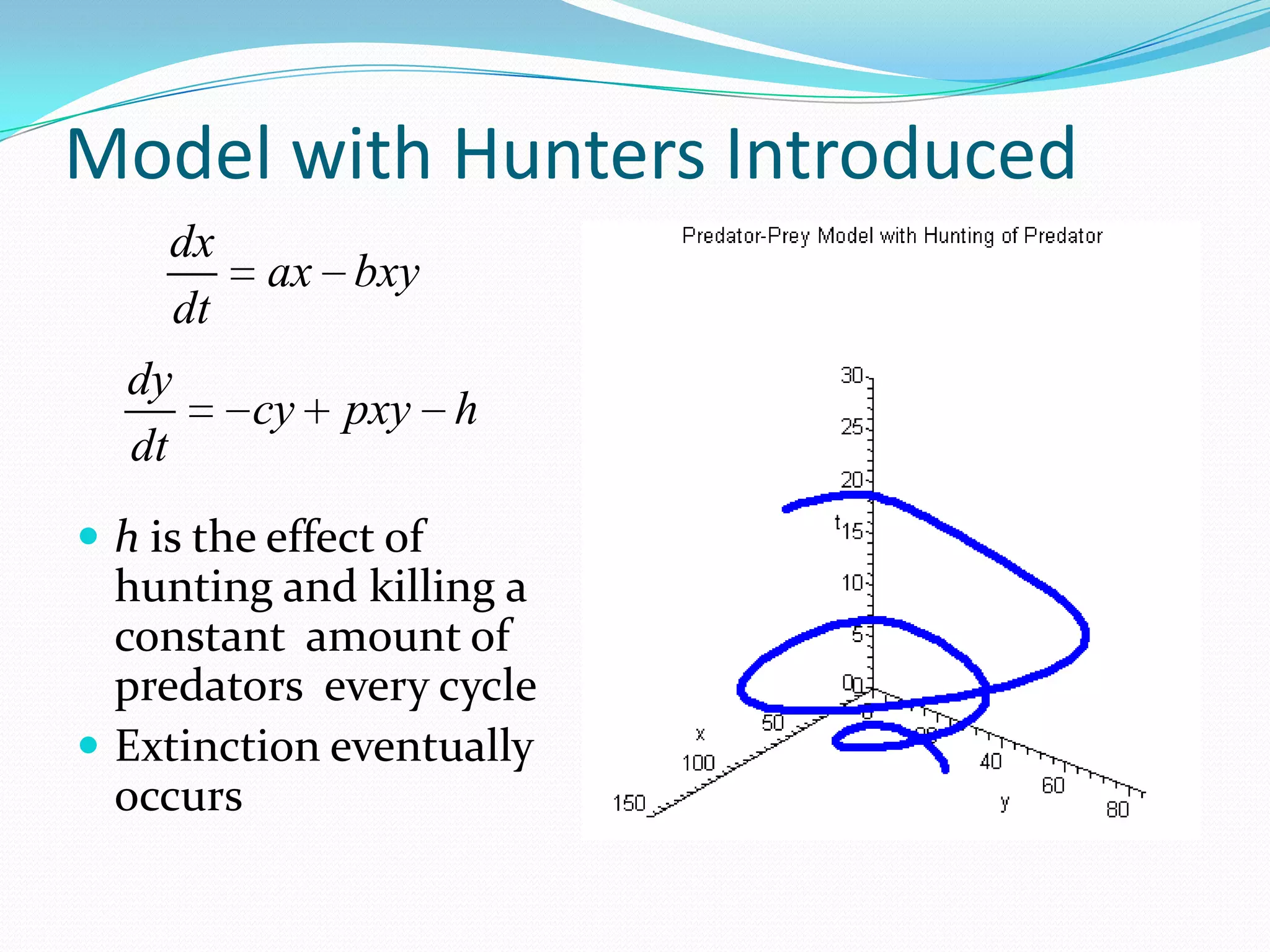
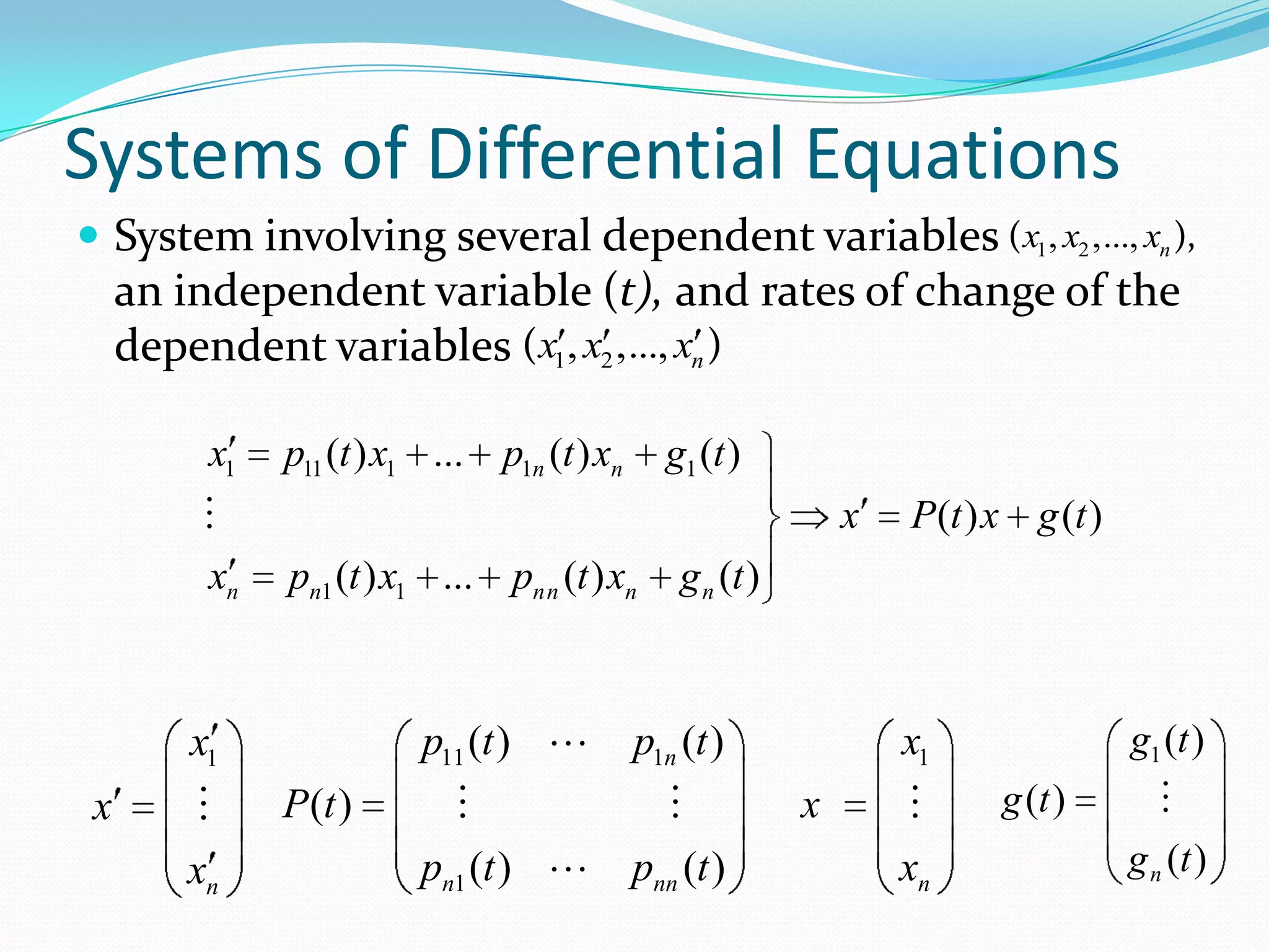
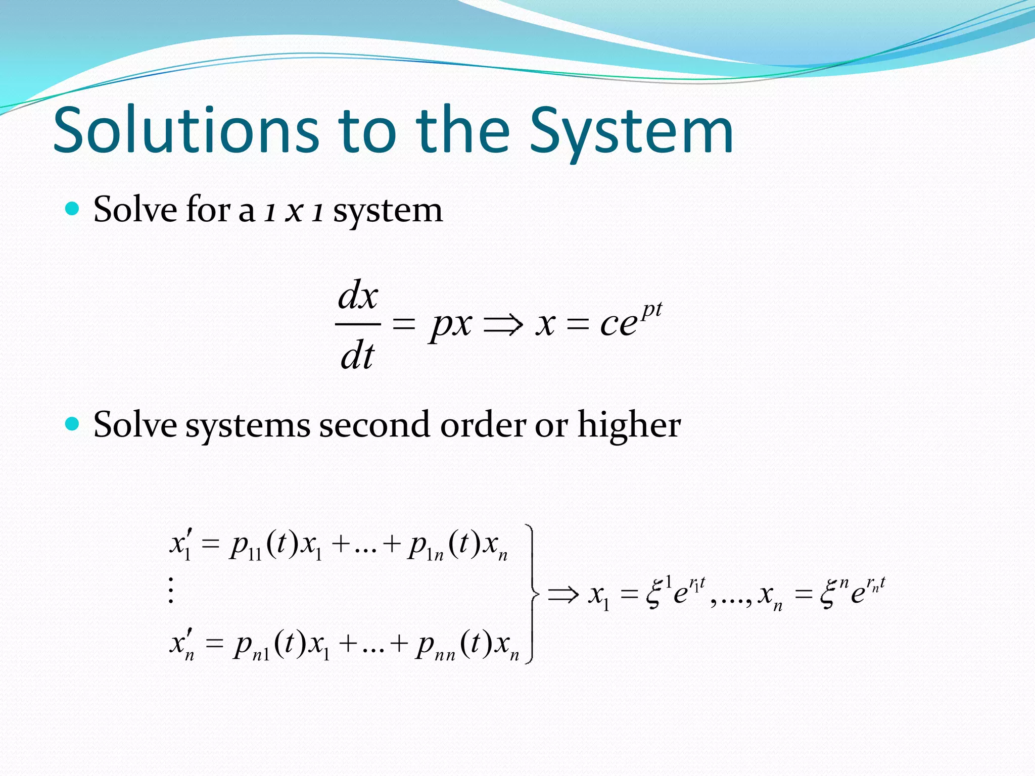
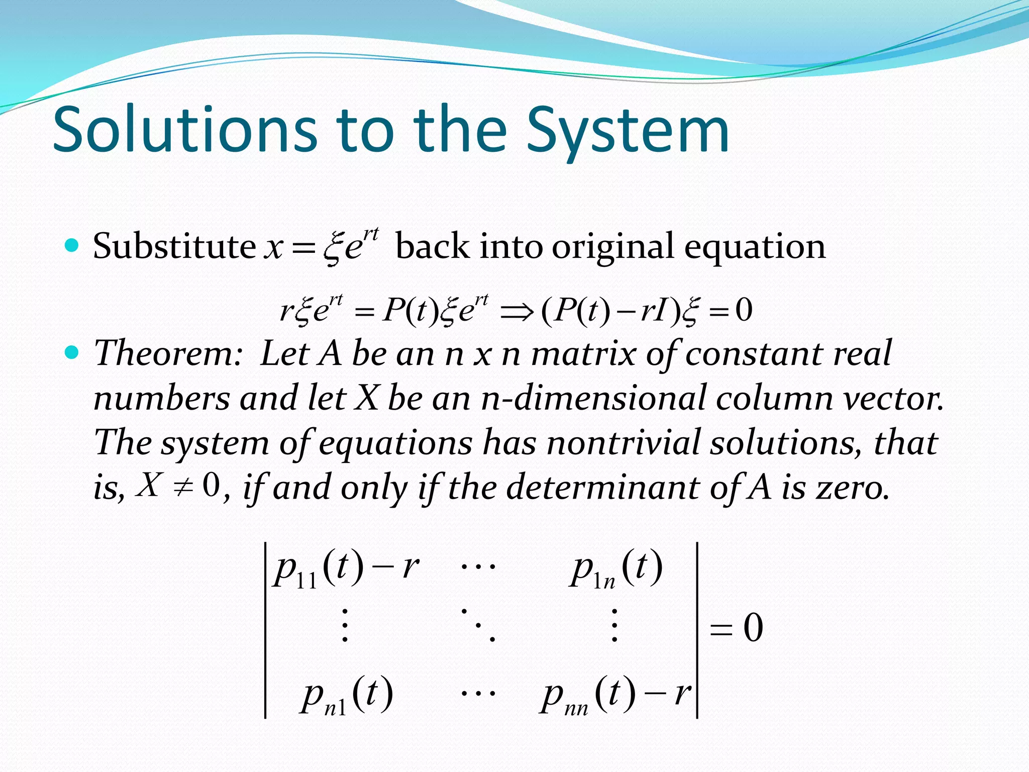
Presentation by: Joshua Dagenais
Systems of Differential Equations
 System involving several dependent variables ( x1, x2 ,..., xn ),
     an independent variable (t), and rates of change of the
     dependent variables ( x1, x2 ,..., xn )

         x1   p11 (t ) x1 ... p1n (t ) xn     g1 (t )
                                                              x   P(t ) x g (t )
         xn   pn1 (t ) x1 ... pnn (t ) xn       g n (t )


        x1              p11 (t )           p1n (t )               x1               g1 (t )
 x           P (t )                                     x            g (t )        
        xn              pn1 (t )           pnn (t )               xn               g n (t )
Solutions to the System
 Solve for a 1 x 1 system

                      dx                           pt
                               px         x   ce
                      dt
 Solve systems second order or higher


       x1   p11 (t ) x1 ... p1n (t ) xn
                                                        1 r1t         n rn t
                                             x1         e ,..., xn    e
       xn   pn1 (t ) x1 ... pnn (t ) xn
Solutions to the System
                      rt
 Substitute x       e back into original equation
             r ert         P(t ) ert   ( P(t ) rI )   0
 Theorem: Let A be an n x n matrix of constant real
 numbers and let X be an n-dimensional column vector.
 The system of equations has nontrivial solutions, that
 is, X 0 , if and only if the determinant of A is zero.

             p11 (t ) r                 p1n (t )
                                                   0
                 pn1 (t )             pnn (t ) r
Solutions to the System
 Solving the determinant gives the characteristic eqn.
              a0r n a1r n 1 ... an 1r an 0
 The roots , r, are the Eigenvalues r1 ,..., rn .
 Eigenvalues are used to solve for the associated
  Eigenvectors, 1 ,..., n , and the specific solutions
                                   n rnt
  x(1) (t ) 1er1t ,..., x( n) (t )  e
 Specific solutions as a general solution


          (1)               (k )          (1)      ( n)
  x c1x (t )  ck x (t ) if W[ x ,..., x ] 0
Eigenvalues (Real & Distinct)
 Eigenvalues are of opposite signs,
 the origin is a saddle point, and
 trajectories are asymptotic to the
 Eigenvectors
                                        1       t        2
                             x(t ) c1       e       c2       e 2t
                                        2                1


 Eigenvalues are of the same signs, the
 the origin is a node, and trajectories
 converge to origin if Eigenvalues are
 negative and vice versa if positive
                                     7 1 4t          3 1 2t
                             x(t )       e               e
                                     2 1            2 3
Eigenvalues (Complex)
 Eigenvalues are complex with a
  nonzero real point (a+bi)
 Use one of Euler’s Formulas
  e( i )t e t cos( t ) i e t sin( t )
  to find real-valued solutions
 The origin is called a spiral point
  and trajectories converge to origin
  if Eigenvalues are negative and vice
  versa if positive
                                                          cos(2t )                   sin(2t )
                                        x(t ) c1et                       c2et
                                                     sin(2t ) cos(2t )          sin(2t ) cos(2t )
Eigenvalues (Repeated)
 Eigenvalues are real and
  repeated with multiplicity 2
 Use x(t ) tert     ert to solve
  for the specific solution of
  second repeated Eigenvalue
 The origin is called a improper
  node and trajectories converge
   to origin if Eigenvalues are         x(t ) c1
                                                   1
                                                   2
                                                       e6t c2
                                                                1
                                                                2
                                                                    t
                                                                        0
                                                                        1
                                                                            e6t


  negative and vice versa if positive
Application
 Predator-Prey Model also
  known as the Lokta-Volterra
  Model
 Part of mathematical ecology
  that studies populations that
  interact, thereby affecting each
  other's growth rates
 Model represents the "natural"
  growth rate and the "carrying
  capacity" of the environment
  (predators & prey)
Predator-Prey Model
 Few interactions have been
  recorded in nature
 One such set of data was
  taken between the
  Snowshoe Hare and the
  Canadian Lynx for almost
  100 years
 The dominating feature is
  the oscillation behavior of
  both populations
Predator-Prey Assumptions
 x(t) will represent the number of prey at a time given
  by t and y(t) will represent the number of predators at
  a time also given by t.
 In the absence of the predator, the prey grows at a rate
  proportional to the current population; thus
   dx
        ax, a 0, when y 0
   dt
 In the absence of the prey, the predator dies out; thus
  dy
        cy, c   0, when x   0
  dt
Predator-Prey Assumptions
 The number of encounters between predator and prey
  is proportional to the product of their populations
 The growth rate of the predator is increased by a term
  of the form bxy, while the growth rate of the prey is
  decreased by a term –pxy
  dx                            dy
       ax bxy    x(a by ) and        cy   pxy     y( c   px)
  dt                            dt

 Critical points (when x(a by)      0 and y( c     px) 0)
 are (0,0) and (c / p, a / b)
Predator-Prey Example
 dx
        x 0.03 xy
 dt
dy
       0.4 y 0.01xy
dt
     a 1, b 0.03

 c 0.4, p 0.01

 cp    (40,100 3)     1 ln y 0.03 y 0.4 ln x 0.01 x C
Predator-Prey Example
 For
   x(0) 15 and y(0) 15
 The predator (green)
  population lags
  behind the prey (blue)
 Population for both
  populations are
  periodic (in this case
  about a periodicity of
  t=11)
Predator-Prey Example
 Population of predators vs.
    prey as t       for
    x(0) 15 and y(0) 15
   Prey first increase because
    of small population
   Predators increase because
    of abundance of food
   Heavier predation causes
    prey to decrease
   Predators decrease because
    of diminished food supply
   Cycle repeats itself
Predator-Prey Example
 Analysis of the Nonzero Critical Point c p   (40,100 3)
Predator-Prey Example
 Analysis of the Nonzero Critical Point c p   (40,100 3)
Model with Hunters Introduced
     dx
           ax bxy
     dt
  dy
          cy   pxy h
  dt
 h is the effect of
  hunting and killing a
  constant amount of
  predators every cycle
 Extinction eventually
  occurs

Systems Of Differential Equations

  • 1.
  • 2.
    Systems of DifferentialEquations  System involving several dependent variables ( x1, x2 ,..., xn ), an independent variable (t), and rates of change of the dependent variables ( x1, x2 ,..., xn ) x1 p11 (t ) x1 ... p1n (t ) xn g1 (t )  x P(t ) x g (t ) xn pn1 (t ) x1 ... pnn (t ) xn g n (t ) x1 p11 (t )  p1n (t ) x1 g1 (t ) x  P (t )   x  g (t )  xn pn1 (t )  pnn (t ) xn g n (t )
  • 3.
    Solutions to theSystem  Solve for a 1 x 1 system dx pt px x ce dt  Solve systems second order or higher x1 p11 (t ) x1 ... p1n (t ) xn 1 r1t n rn t  x1 e ,..., xn e xn pn1 (t ) x1 ... pnn (t ) xn
  • 4.
    Solutions to theSystem rt  Substitute x e back into original equation r ert P(t ) ert ( P(t ) rI ) 0  Theorem: Let A be an n x n matrix of constant real numbers and let X be an n-dimensional column vector. The system of equations has nontrivial solutions, that is, X 0 , if and only if the determinant of A is zero. p11 (t ) r  p1n (t )    0 pn1 (t )  pnn (t ) r
  • 5.
    Solutions to theSystem  Solving the determinant gives the characteristic eqn. a0r n a1r n 1 ... an 1r an 0  The roots , r, are the Eigenvalues r1 ,..., rn .  Eigenvalues are used to solve for the associated Eigenvectors, 1 ,..., n , and the specific solutions n rnt x(1) (t ) 1er1t ,..., x( n) (t ) e  Specific solutions as a general solution (1) (k ) (1) ( n) x c1x (t )  ck x (t ) if W[ x ,..., x ] 0
  • 6.
    Eigenvalues (Real &Distinct)  Eigenvalues are of opposite signs, the origin is a saddle point, and trajectories are asymptotic to the Eigenvectors 1 t 2 x(t ) c1 e c2 e 2t 2 1  Eigenvalues are of the same signs, the the origin is a node, and trajectories converge to origin if Eigenvalues are negative and vice versa if positive 7 1 4t 3 1 2t x(t ) e e 2 1 2 3
  • 7.
    Eigenvalues (Complex)  Eigenvaluesare complex with a nonzero real point (a+bi)  Use one of Euler’s Formulas e( i )t e t cos( t ) i e t sin( t ) to find real-valued solutions  The origin is called a spiral point and trajectories converge to origin if Eigenvalues are negative and vice versa if positive cos(2t ) sin(2t ) x(t ) c1et c2et sin(2t ) cos(2t ) sin(2t ) cos(2t )
  • 8.
    Eigenvalues (Repeated)  Eigenvaluesare real and repeated with multiplicity 2  Use x(t ) tert ert to solve for the specific solution of second repeated Eigenvalue  The origin is called a improper node and trajectories converge to origin if Eigenvalues are x(t ) c1 1 2 e6t c2 1 2 t 0 1 e6t negative and vice versa if positive
  • 9.
    Application  Predator-Prey Modelalso known as the Lokta-Volterra Model  Part of mathematical ecology that studies populations that interact, thereby affecting each other's growth rates  Model represents the "natural" growth rate and the "carrying capacity" of the environment (predators & prey)
  • 10.
    Predator-Prey Model  Fewinteractions have been recorded in nature  One such set of data was taken between the Snowshoe Hare and the Canadian Lynx for almost 100 years  The dominating feature is the oscillation behavior of both populations
  • 11.
    Predator-Prey Assumptions  x(t)will represent the number of prey at a time given by t and y(t) will represent the number of predators at a time also given by t.  In the absence of the predator, the prey grows at a rate proportional to the current population; thus dx ax, a 0, when y 0 dt  In the absence of the prey, the predator dies out; thus dy cy, c 0, when x 0 dt
  • 12.
    Predator-Prey Assumptions  Thenumber of encounters between predator and prey is proportional to the product of their populations  The growth rate of the predator is increased by a term of the form bxy, while the growth rate of the prey is decreased by a term –pxy dx dy ax bxy x(a by ) and cy pxy y( c px) dt dt  Critical points (when x(a by) 0 and y( c px) 0) are (0,0) and (c / p, a / b)
  • 13.
    Predator-Prey Example dx x 0.03 xy dt dy 0.4 y 0.01xy dt a 1, b 0.03 c 0.4, p 0.01 cp (40,100 3) 1 ln y 0.03 y 0.4 ln x 0.01 x C
  • 14.
    Predator-Prey Example  For x(0) 15 and y(0) 15  The predator (green) population lags behind the prey (blue)  Population for both populations are periodic (in this case about a periodicity of t=11)
  • 15.
    Predator-Prey Example  Populationof predators vs. prey as t for x(0) 15 and y(0) 15  Prey first increase because of small population  Predators increase because of abundance of food  Heavier predation causes prey to decrease  Predators decrease because of diminished food supply  Cycle repeats itself
  • 16.
    Predator-Prey Example Analysisof the Nonzero Critical Point c p (40,100 3)
  • 17.
    Predator-Prey Example Analysisof the Nonzero Critical Point c p (40,100 3)
  • 18.
    Model with HuntersIntroduced dx ax bxy dt dy cy pxy h dt  h is the effect of hunting and killing a constant amount of predators every cycle  Extinction eventually occurs