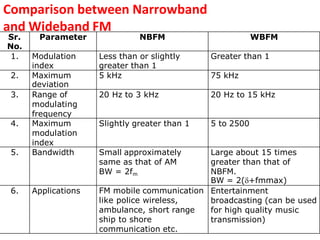
This document provides an overview of analog communication systems and focuses on angle modulation techniques, specifically frequency modulation (FM) and phase modulation (PM). It defines these modulation techniques and discusses key concepts such as modulation index, frequency deviation, bandwidth, and Carson's rule for calculating FM bandwidth. Narrowband FM is used for applications requiring a small bandwidth like short-range communications, while wideband FM is used for entertainment broadcasting where higher quality transmission is needed and bandwidth is not a constraint. FM can be represented in either the time domain by showing the continuous variation of the carrier signal over time, or in the frequency domain using a spectrum that plots the amplitudes of the carrier and sideband frequencies.

1. ANALOG COMMUNICATION SYSTEMS
By
Ms. Swati Shrrpal Halunde
Assistant Professor DEPT. of
E.C.E S.I.T.C.O.E. Yadrav-
Ichalkaranji
ANGLE MODULATION

2. ANGLE MODULATION
Angle modulation is a process
carrier in accordance with the
modulating signal.
of varying angle of the
instantaneous values of
Angle can be varied by varying frequency or phase.
Angle modulation is of 2 types.
• Frequency Modulation
• Phase Modulation

3. Frequency Modulation
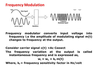
The process of varying frequency of
accordance with the instantaneous values of
the carrier in
the
modulating signal.
Relation between angle and frequency :
Consider carrier signal c(t)= Ac Cos (wct+φ)
= Ac Cos (2πfct +φ)
Where, Wc= Carrier frequency
φ = Phase
C(t) = Ac Cos[ψ(t)], where, ψ(t)= wct+φ
i.e Frequency can be obtained by derivating angle and
angle can be obtained by integrating frequency.

4. Frequency Modulation
Frequency modulator converts input voltage into
frequency i.e the amplitude of modulating signal m(t)
changes to frequency at the output.
Consider carrier signal c(t) =Ac Coswct
The frequency variation at the output is called
instantaneous frequency and is expressed as,
wi = wc + kf m(t)
Where, kf = frequency sensitivity factor in Hz/volt

5. Frequency Modulation
The angle of the carrier
written as,
after modulation can be
Frequency modulated signal can be written as,
AFM(t) = Ac Cos [ψi(t)] = Ac Cos [wct + kfʃm(t)dt]
Frequency Deviation in FM:
The instantaneous frequency, wi = wc + kf m(t)
= wc + Δw
Where, Δw = kf m(t) is called frequency deviation which
may be positive or negative depending on the sign of
m(t).

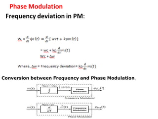
6. Phase Modulation
The process of varying the phase of carrier in accordance
with instantaneous values of the modulating signal.
Consider modulating signal x(t) and carrier signal c(t) =
Ac Coswct
Phase modulating signal,
APM(t) = Ac Cos[ ψi(t)]
Where, ψi(t) = wct + kpm(t)
Where, kp = Phase sensitivity factor in rad/volt
APM(t) = Ac Cos[wct + kpm(t)]

7. Phase Modulation
Frequency deviation in PM:
Conversion between Frequency and Phase Modulation:

8. Modulation Index
Definition:
Modulation Index is defined as the ratio of frequency
deviation () to the modulating frequency (fm).
M.I.=Frequency Deviation
Modulating Frequency
mf =δ
fm
In FM M.I.>1
Modulation Index of FM decides −
(i)Bandwidth of the FM wave.
(ii)Number of sidebands in FM wave.

9. Deviation Ratio
The modulation index corresponding to maximum deviation
and maximum modulating frequency is called deviation ratio.
Deviation Ratio= Maximum Deviation
Maximum modulating Frequency
= δmax
fmax
In FM broadcasting the maximum value of deviation is limited to 75
kHz. The maximum modulating frequency is also limited to 15 kHz.

10. Percentage M.I. of FM
The percentage modulation is defined as the ratio of the
actual frequency deviation produced by the modulating signal
to the maximum allowable frequency deviation.
% M.I = Actual deviation
Maximum allowable deviation


11. Frequency Spectrum of FM
Frequency spectrum is a graph of amplitude versus frequency.
The frequency spectrum of FM wave tells us about number of
sideband present in the FM wave and their amplitudes.
The expression for FM wave is not simple. It is complex because it
is sine of sine function.
Only solution is to use ‘Bessels Function’.
Equation (2.32) may be expanded as,
eFM = {A J0 (mf) sin ct
+ J1 (mf) [sin (c + m) t − sin (c − m) t]
+ J1 (mf) [sin (c + 2m) t + sin (c − 2m) t]
+ J3 (mf) [sin (c + 3m) t − sin (c − 3m) t]
+ J4 (mf) [sin (c + 4m) t + sin (c − 4m) t]
+ }  (2.33)
From this equation it is seen that the FM wave consists of:
(i)Carrier (First term in equation).
(ii)Infinite number of sidebands (All terms except first term are
sidebands).
The amplitudes of carrier and sidebands depend on ‘J’ coefficient.
c = 2fc, m = 2fm
So in place of c and m, we can use fc and fm.

12. Fig. : Ideal Frequency Spectrum of FM

13. Bandwidth of FM
From frequency spectrum of FM wave shown in Fig.
2.26, we can say that the bandwidth of FM wave is
infinite.
But practically, it is calculated based on how many
sidebands have significant amplitudes.
(i)The Simple Method to calculate the bandwidth is −
BW=2fmx Number of significant sidebands --(1)
With increase in modulation index, the number of
significant sidebands increases. So that bandwidth also
increases.
(ii)The second method to calculate bandwidth is by
Carson’s rule.

14. Carson’s rule states that, the bandwidth of FM wave is twice
the sum of deviation and highest modulating frequency.
BW=2( +fmmax) (2)
Highest order side band = To be found from table 2.1 after the
calculation of modulation Index m where, m = /fm
e.g. If m= 20KHZ/5KHZ
From table, for modulation index 4, highest order side band is 7th.
Therefore, the bandwidth is
B.W. = 2 fm  Highest order side band
=2  5 kHz  7
=70 kHz

15. Types of Frequency Modulation
FM (Frequency Modulation)
Narrowband
FM (NBFM)
[Whenmodulation indexissmall]
WidebandFM
(WBFM)
[Whenmodulationindexislarge]

16. Comparison between Narrowband
and Wideband FM
Sr.
No.
Parameter NBFM WBFM
1. Modulation
index
Less than or slightly
greater than 1
Greater than 1
2. Maximum
deviation
5 kHz 75 kHz
3. Range of
modulating
frequency
20 Hz to 3 kHz 20 Hz to 15 kHz
4. Maximum
modulation
index
Slightly greater than 1 5 to 2500
5. Bandwidth Small approximately
same as that of AM
BW = 2fm
Large about 15 times
greater than that of
NBFM.
BW = 2(+fmmax)
6. Applications FM mobile communication
like police wireless,
ambulance, short range
ship to shore
communication etc.
Entertainment
broadcasting (can be used
for high quality music
transmission)

17. Representation of FM
FM can be represented by two ways:
1. Time domain.
2. Frequency domain.
1.FM in Time Domain
Time domain representation means continuous variation of voltage with respect
to time as shown in Fig. .
Fig. 1 FM in Time Domain
2.FM in Frequency Domain
• Frequency domain is also known as frequency spectrum.
• FM in frequency domain means graph or plot of amplitude versus frequency as
shown in Fig. 2.29.
Fig. 2: FM in Frequency Domain