Frequency modulation

1. QUENCY MODULATION
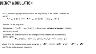
In FM, the message signal m(t) controls the frequency fc of the carrier. Consider the
carrier
then for FM we may write:
FM signal ,where the frequency deviation
will depend on m(t).
Given that the carrier frequency will change we may write for an instantaneous
carrier signal
where i is the instantaneous angle =
and fi is the instantaneous frequency.
𝑣 𝑐 ( 𝑡 )= 𝑉 𝑐 cos ( ω𝑐 𝑡 )
𝑣 𝑠 (𝑡 )=𝑉 𝑐 cos (2 π ( 𝑓 𝑐+ frequency deviation ) 𝑡 )
𝑉 𝑐 cos (ω𝑖 𝑡)=𝑉 𝑐 cos (2 π 𝑓 𝑖 𝑡)=𝑉 𝑐 cos ( φ𝑖)
ω 𝑖 𝑡 =2 π 𝑓 𝑖 𝑡

2. QUENCY MODULATION
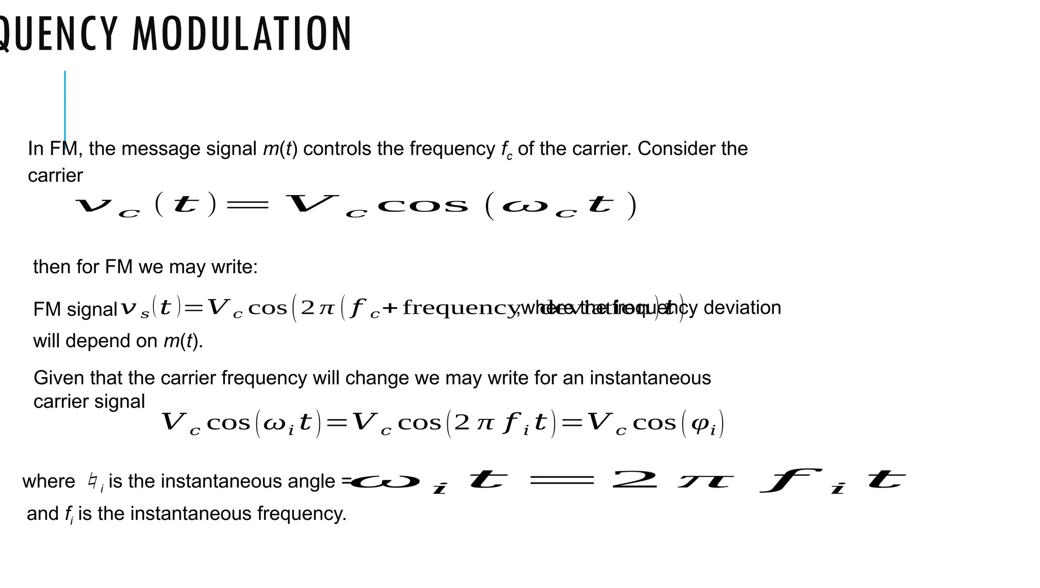
Since then
i.e. frequency is proportional to the rate of change of angle.
If fc is the unmodulated carrier and fm is the modulating frequency, then we may
deduce that
fc is the peak deviation of the carrier.
Hence, we have
,i.e.
φ𝑖=2 π 𝑓 𝑖 𝑡
𝑑 φ𝑖
𝑑𝑡
= 2 π 𝑓 𝑖 or 𝑓 𝑖=
1
2 π
𝑑 φ𝑖
𝑑𝑡
𝑓 𝑖 = 𝑓 𝑐 + Δ 𝑓 𝑐 cos (ω𝑚 𝑡 )=
1
2 π
𝑑 φ𝑖
𝑑𝑡
1
2π
𝑑 φ𝑖
𝑑𝑡
= 𝑓 𝑐 + Δ 𝑓 𝑐 cos(ω𝑚 𝑡)

3. FREQUENCY MODULATION
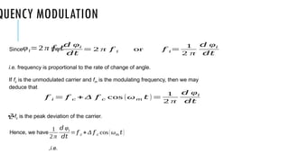
After integration i.e.
Hence for the FM signal,
∫(ω𝑐 +2 πΔ 𝑓 𝑐 cos(ω𝑚 𝑡)) 𝑑𝑡
φ 𝑖= ω𝑐 𝑡 +
2 πΔ 𝑓 𝑐 sin (ω𝑚 𝑡 )
ω𝑚
φ 𝑖= ω𝑐 𝑡 +
Δ 𝑓 𝑐
𝑓 𝑚
sin ( ω𝑚 𝑡 )
𝑣 𝑠(𝑡 )=𝑉 𝑐 cos(φ𝑖 )
𝑣 𝑠 (𝑡 )=𝑉 𝑐 cos
(ω𝑐 𝑡 +
Δ 𝑓 𝑐
𝑓 𝑚
sin ( ω𝑚𝑡 ))

4. FREQUENCY MODULATION
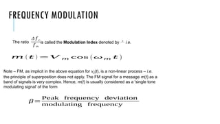
The ratio is called the Modulation Index denoted by  i.e.
Note – FM, as implicit in the above equation for vs(t), is a non-linear process – i.e.
the principle of superposition does not apply. The FM signal for a message m(t) as a
band of signals is very complex. Hence, m(t) is usually considered as a 'single tone
modulating signal' of the form
Δ 𝑓 𝑐
𝑓 𝑚
β=
Peak frequency deviation
modulating frequency
𝑚 ( 𝑡 ) =𝑉 𝑚 cos (ω𝑚 𝑡 )

5. FREQUENCY MODULATION
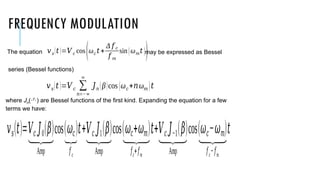
The equation may be expressed as Bessel
series (Bessel functions)
where Jn() are Bessel functions of the first kind. Expanding the equation for a few
terms we have:
𝑣𝑠(𝑡)=𝑉𝑐 𝐽0(𝛽)
⏟
Amp
cos(𝜔𝑐)
⏟
𝑓𝑐
𝑡+𝑉𝑐 𝐽1(𝛽)
⏟
Amp
cos(𝜔𝑐+𝜔𝑚)
⏟
𝑓𝑐
+𝑓𝑚
𝑡+𝑉𝑐 𝐽−1(𝛽)
⏟
Amp
cos(𝜔𝑐−𝜔𝑚)
⏟
𝑓𝑐
−𝑓𝑚
𝑡
𝑣𝑠(𝑡 )=𝑉𝑐 cos
(ω𝑐 𝑡 +
Δ 𝑓 𝑐
𝑓 𝑚
sin(ω𝑚𝑡 ))
𝑣𝑠(𝑡)=𝑉𝑐 ∑
𝑛=−∞
∞
𝐽𝑛 (β)cos (ω𝑐+𝑛ω𝑚 )𝑡

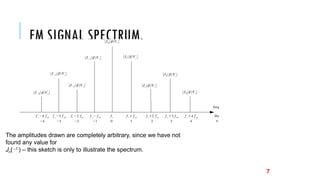
6. FM SIGNAL SPECTRUM.
The amplitudes drawn are completely arbitrary, since we have not
found any value for
Jn() – this sketch is only to illustrate the spectrum.
7

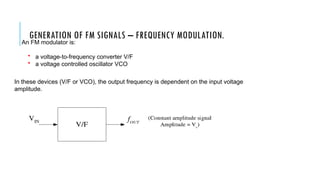
7. GENERATION OF FM SIGNALS – FREQUENCY MODULATION.
An FM modulator is:
• a voltage-to-frequency converter V/F
• a voltage controlled oscillator VCO
In these devices (V/F or VCO), the output frequency is dependent on the input voltage
amplitude.

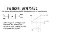
8. FM SIGNAL WAVEFORMS.
The diagrams below illustrate FM signal waveforms for various inputs
At this stage, an input digital data
sequence, d(t), is introduced –
the output in this case will be FSK,
(Frequency Shift Keying).

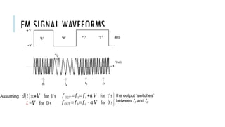
9. FM SIGNAL WAVEFORMS.
Assuming 𝑑(𝑡)=+𝑉 for 1′s
¿−𝑉 for 0′s
𝑓 𝑂𝑈𝑇 =𝑓 1=𝑓 𝑐+𝛼𝑉 for 1′s
𝑓 𝑂𝑈𝑇 =𝑓 0=𝑓 𝑐 −𝛼𝑉 for 0′s}the output ‘switches’
between f1 and f0.

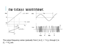
10. FM SIGNAL WAVEFORMS.
The output frequency varies ‘gradually’ from fc to (fc + Vm), through fc to
(fc - Vm) etc.

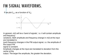
11. FM SIGNAL WAVEFORMS.
If we plot fOUT as a function of VIN:
In general, m(t) will be a ‘band of signals’, i.e. it will contain amplitude
and frequency
variations. Both amplitude and frequency change in m(t) at the input
are translated to
(just) frequency changes in the FM output signal, i.e. the amplitude of
the output FM
signal is constant.
Amplitude changes at the input are translated to deviation from the
carrier at the
output. The larger the amplitude, the greater the deviation.

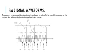
12. FM SIGNAL WAVEFORMS.
Frequency changes at the input are translated to rate of change of frequency at the
output. An attempt to illustrate this is shown below:

13. FM SPECTRUM – BESSEL COEFFICIENTS.
The FM signal spectrum may be
determined from
𝑣𝑠(𝑡)=𝑉𝑐 ∑
𝑛=−∞
∞
𝐽𝑛(𝛽)cos(¿𝜔𝑐+𝑛𝜔𝑚)𝑡¿
The values for the Bessel coefficients, Jn() may be
found from
graphs or, preferably, tables of ‘Bessel functions of the
first kind’.

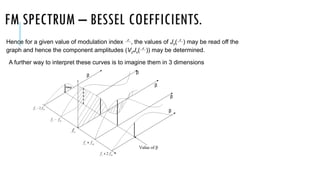
14. FM SPECTRUM – BESSEL COEFFICIENTS.
Hence for a given value of modulation index , the values of Jn() may be read off the
graph and hence the component amplitudes (VcJn()) may be determined.
A further way to interpret these curves is to imagine them in 3 dimensions

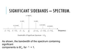
15. SIGNIFICANT SIDEBANDS – SPECTRUM.
As shown, the bandwidth of the spectrum containing
significant
components is 6fm, for  = 1.

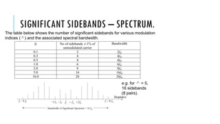
16. SIGNIFICANT SIDEBANDS – SPECTRUM.
The table below shows the number of significant sidebands for various modulation
indices () and the associated spectral bandwidth.
 No of sidebands 1% of
unmodulated carrier
Bandwidth
0.1 2 2fm
0.3 4 4fm
0.5 4 4fm
1.0 6 6fm
2.0 8 8fm
5.0 16 16fm
10.0 28 28fm
e.g. for  = 5,
16 sidebands
(8 pairs).

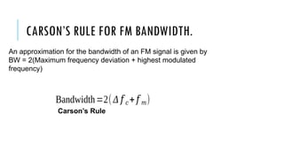
17. CARSON’S RULE FOR FM BANDWIDTH.
An approximation for the bandwidth of an FM signal is given by
BW = 2(Maximum frequency deviation + highest modulated
frequency)
Bandwidth=2(Δ 𝑓 𝑐+𝑓 𝑚)
Carson’s Rule

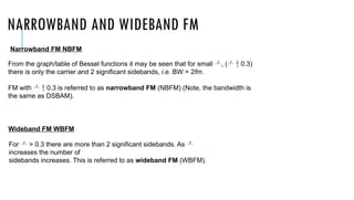
18. NARROWBAND AND WIDEBAND FM
From the graph/table of Bessel functions it may be seen that for small , (  0.3)
there is only the carrier and 2 significant sidebands, i.e. BW = 2fm.
FM with   0.3 is referred to as narrowband FM (NBFM) (Note, the bandwidth is
the same as DSBAM).
For  > 0.3 there are more than 2 significant sidebands. As 
increases the number of
sidebands increases. This is referred to as wideband FM (WBFM).
Narrowband FM NBFM
Wideband FM WBFM

19. APPLICATIONS
•FM Radio Broadcasting: This is the most common
application of FM, particularly for music and high-
fidelity audio broadcasts. FM broadcasting utilizes the
VHF band (typically 88 to 108 MHz) and offers better
sound quality and reduced interference compared to AM
radio.
•Television Sound: In analog television broadcasting, FM
was employed for transmitting the audio signal alongside
the video signal, which was typically transmitted using
AM.
•Satellite TV: Some satellite television broadcasts also
utilize FM for transmitting video signals to receiver
stations.
1. Broadcasting

20. APPLICATIONS
•Two-Way Radio Communication: Narrowband FM
(NBFM) is commonly used in two-way radio
communication systems, including police radios, amateur
radio, and various mobile communication applications.
•Wireless Technologies: FM is integral to various wireless
communication systems, such as Bluetooth and other
technologies that transmit data over radio waves.
•Data Transmission: FM facilitates the transfer of digital
data over radio waves by modulating the carrier wave's
frequency based on the digital signal.
2. Telecommunications

21. APPLICATIONS
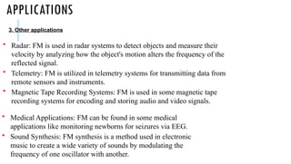
• Medical Applications: FM can be found in some medical
applications like monitoring newborns for seizures via EEG.
• Sound Synthesis: FM synthesis is a method used in electronic
music to create a wide variety of sounds by modulating the
frequency of one oscillator with another.
3. Other applications
• Radar: FM is used in radar systems to detect objects and measure their
velocity by analyzing how the object's motion alters the frequency of the
reflected signal.
• Telemetry: FM is utilized in telemetry systems for transmitting data from
remote sensors and instruments.
• Magnetic Tape Recording Systems: FM is used in some magnetic tape
recording systems for encoding and storing audio and video signals.

22. Madhav Institute
of
Technology
&
Science
Gwalior (M.P.)
(Deemed to be
University)
THANK YOU