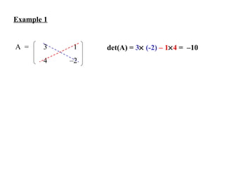
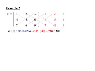
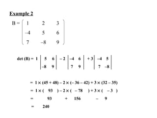
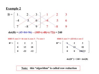
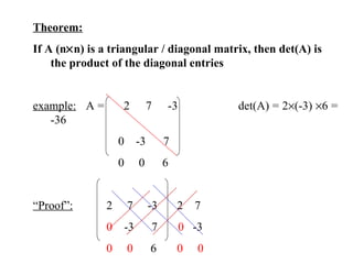
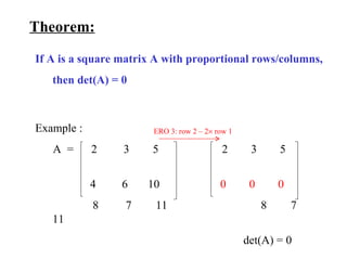
This document summarizes key concepts about determinants including: 1) The determinant function maps a square matrix to a real number and can be evaluated through cofactor expansion or row reduction. 2) Properties of the determinant include being zero if a row or column is zero and being the product of diagonals for triangular matrices. 3) Elementary row operations preserve the determinant up to a factor of -1 for row interchanges. 4) Cramer's rule uses determinants to solve systems of linear equations when the matrix is invertible.

1. CHAPTER 2 – DETERMINANTS 2.1. The Determinant Function 2.2. Evaluating Determinants by Row Reduction 2.3. Properties of the Determinant Function 2.4. Cofactor Expansion; Cramer’s Rule

2. The determinant function is a real-valued function of a matrix variable input : matrix output : real number

3. Example 1 A = 3 1 4 –2 det(A) = 3  (-2) – 1  4 = –10

4. Example 2 B = 1 2 3 1 2 3 -4 5 6 -4 5 6 7 -8 9 7 -8 9 det(B) = (45+84+96) – (105+(-48)+(-72)) = 240

5. Example 2 B = 1 2 3 – 4 5 6 7 –8 9 det (B) = 1 5 6 – 2 –4 6 + 3 –4 5 – 8 9 7 9 7 –8 = 1  (45 + 48) – 2  (– 36 – 42) + 3  (32 – 35) = 1  ( 93 ) – 2  ( – 78 ) + 3  ( – 3 ) = 93 + 156 – 9 = 240

6. Theorem: Let A be a square matrix. If A has a row/column of zeros, then det(A) = 0 Det(A) = det(A T ) Example B = 1 2 3 1 2 3 0 0 0 0 0 0 7 -8 9 7 -8 9 det(B) = 0

7. Theorem: If A (n  n) is a triangular / diagonal matrix, then det(A) is the product of the diagonal entries example: A = 2 7 -3 det(A) = 2  (-3)  6 = -36 0 -3 7 0 0 6 “ Proof”: 2 7 -3 2 7 0 -3 7 0 -3 0 0 6 0 0

8. Theorem: If a square matrix A is transformed into matrix B by ERO 1: then det(B) = k  det(A) ERO 2: then det(B) = – det(A) ERO 3: then det(B) = det(A)

9. Example A = 3 1 det (A) = 3  (–2) – 1  4 = – 10 4 –2 ERO 3: row 2 – (4/3)  row 1 A’ = 3 1 det (A’) = – 10 = det(A) 0 –10/3

10. Example 2 B = 1 2 3 1 2 3 – 4 5 6 -4 5 6 7 –8 9 7 –8 9 det(B) = (45+84+96) – (105+(-48)+(-72)) = 240 B’ = 1 2 3 B’’ = 1 2 3 0 13 18 0 13 18 0 -22 -12 0 0 240/13 det(B’’) = 240 = det(B) ERO 3: row 2 + 4  row 1; row 3 – 7  row 1 ERO 3: row 3 + (22/13)  row 2 Note: this “algorithm” is called row reduction

11. Theorem: If A is a square matrix A with proportional rows/columns, then det(A) = 0 Example : A = 2 3 5 2 3 5 4 6 10 0 0 0 8 7 11 8 7 11 det(A) = 0 ERO 3: row 2 – 2  row 1

12. Cramer’s Rule: The solution of a system of linear equation Ax = b where det(A)  0 is unique and is determined by: x j = i = 1, 2, 3, …, n det(A j ) det(A) A j is obtained by replacing the j-th column of matrix A by b

13. How to get the solution space of a system of linear equations Ax = b Gaussian elimination & back substitution Gauss-Jordan elimination Find the inverse A –1 and x = A –1 b Cramer’s Rule

14. Theorem: A square matrix A is invertible iff det(A)  0 If A is an invertible matrix (with inverse A –1 )then det(A –1 ) = 1 / (det(A))

15. Theorem: if A is an (n  n) square matrix, then these are equivalent A is invertible ( A –1 is defined) Ax = 0 has the trivial solution only The reduced row echelon form of A is I n A can be expressed as a product of elementary matrices Ax = b is consistent for every (n  1) matrix b Ax = b has exactly one solution for every (n  1) matrix b Det( A )  0

16. Pelajari sendiri semua definisi, teorema, algoritma yang tidak dibahas di kelas Latihan: 2.1. no. 19 2.2. no. 8 2.3. no. 3 2.4. no. 17