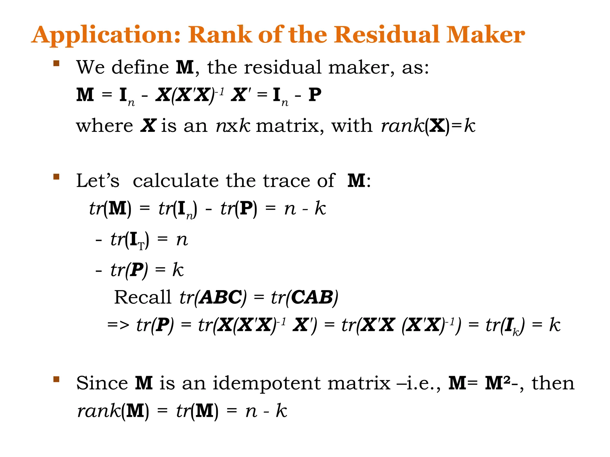
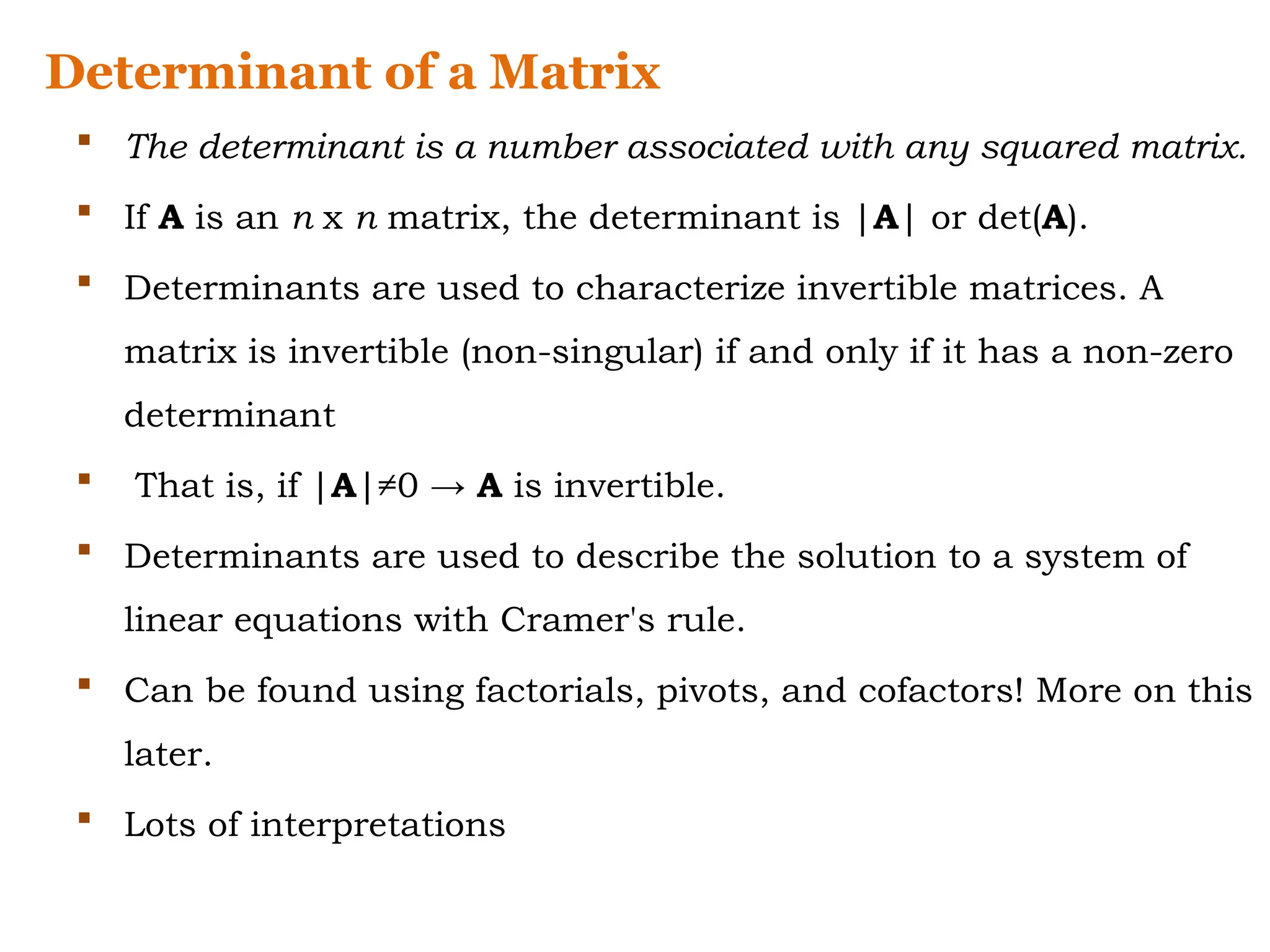
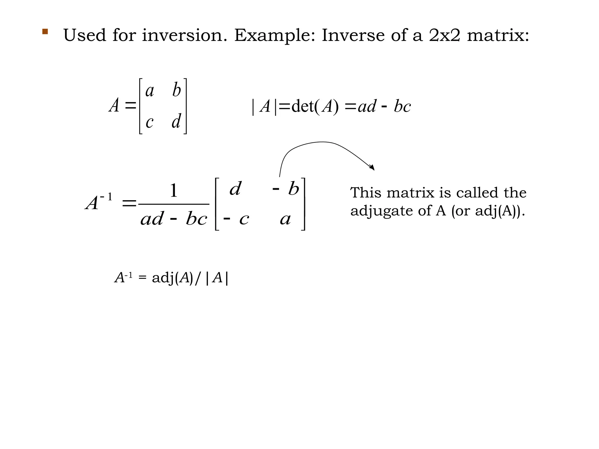
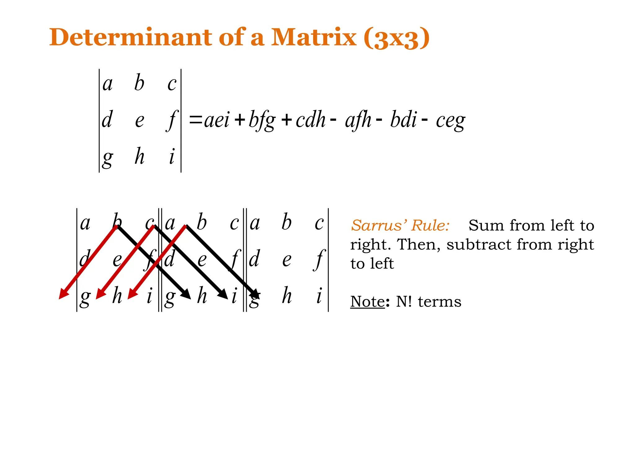
The document discusses the properties and calculations involved in finding the inverse of a matrix, emphasizing that a unique inverse exists only for square matrices. It outlines methods such as Gauss-Jordan elimination and highlights the properties of determinants, including how they relate to the invertibility of matrices. Key concepts like the trace of a matrix and its application in identifying residuals are also reviewed.

1. Determinants
Inverse Matrix
&

2. Inverse matrix
Review
 AA-1
= I
 A-1
A=I
 Necessary for matrix to be square to have unique
inverse.
 If an inverse exists for a square matrix, it is unique
 (A')-1
=(A-1
)‘
 Solution to A x = d
 A-1
A x* = A-1
d
 I x* =A-1
d=> x* = A-1
d(solution depends on A-1
)
 Linear independence a problem to get x*

3. Inverse of a Matrix: Calculation










1
0
0
0
1
0
0
0
1
|
i
h
g
f
e
d
c
b
a
Process:
 Append the identity matrix to A.
 Subtract multiples of the other
rows from the first row to reduce
the diagonal element to 1.
 Transform the identity matrix as
you go.
Theorem: Let A be an invertible (n x n) matrix. Suppose that a
sequence of elementary row-operations reduces A to the identity
matrix. Then the same sequence of elementary row-operations when
applied to the identity matrix yields A-1
.
 When the original matrix is the identity, the identity has become
the inverse!

4. Determination of the Inverse
(Gauss-Jordan Elimination)
AX = I
I X = K
I X = X = A-1
=> K = A-1
1) Augmented matrix
all A, X and I are (n x n)
square matrices
X = A-1
Gauss elimination Gauss-Jordan
elimination
UT: upper triangular
further row
operations
[A I ] [ UT H] [ I K]
2) Transform augmented matrix
Wilhelm Jordan (1842– 1899)

5. Find A-1
using the Gauss-Jordan method.
Gauss-Jordan Elimination: Example 1











2
1
1
1
2
1
1
1
2
A















 












1
0
0
2
1
1
0
1
0
1
2
1
0
0
2
1
2
1
2
1
1
1
0
0
2
1
1
0
1
0
1
2
1
0
0
1
1
1
2
|
.
1 )
2
/
1
(
1
R
I
A






















 

















1
0
2
1
2
3
2
1
0
0
1
2
1
2
1
2
3
0
0
0
2
1
2
1
2
1
1
1
0
0
2
1
1
0
1
0
1
2
1
0
0
2
1
2
1
2
1
1
.
2 )
1
(
&
)
1
( 31
21 R
R
Process:
Expand A|I. Start scaling and adding rows to get I|A-1
.

6. 




















 



















1
0
2
1
2
3
2
1
0
0
3
2
3
1
3
1
1
0
0
0
2
1
2
1
2
1
1
1
0
2
1
2
3
2
1
0
0
1
2
1
2
1
2
3
0
0
0
2
1
2
1
2
1
1
.
3 )
3
/
2
(
2
A
R





















 


















 
1
3
1
3
1
3
4
0
0
0
3
2
3
1
3
1
1
0
0
0
2
1
2
1
2
1
1
1
0
2
1
2
3
2
1
0
0
3
2
3
1
3
1
1
0
0
0
2
1
2
1
2
1
1
.
4 )
2
/
1
(
32
R





















 




















4
3
4
1
4
1
1
0
0
0
3
2
3
1
3
1
1
0
0
0
2
1
2
1
2
1
1
1
3
1
3
1
3
4
0
0
0
3
2
3
1
3
1
1
0
0
0
2
1
2
1
2
1
1
.
5 )
4
/
3
(
3
R

7. 

























 



















 

4
3
4
1
4
1
1
0
0
4
1
4
3
4
1
0
1
0
8
3
8
1
8
5
0
2
1
1
4
3
4
1
4
1
1
0
0
0
3
2
3
1
3
1
1
0
0
0
2
1
2
1
2
1
1
.
6 )
2
/
1
(
&
)
3
/
1
( 13
23 R
R























 























4
3
4
1
4
1
1
0
0
4
1
4
3
4
1
0
1
0
8
2
8
2
8
6
0
0
1
4
3
4
1
4
1
1
0
0
4
1
4
3
4
1
0
1
0
8
3
8
1
8
5
0
2
1
1
.
7 )
2
/
1
(
12
R














































 

4
3
4
1
4
1
4
1
4
3
4
1
4
1
4
1
4
3
4
3
4
1
4
1
1
0
0
4
1
4
3
4
1
0
1
0
8
2
8
2
8
6
0
0
1
|
.
8 1
1
A
A
I

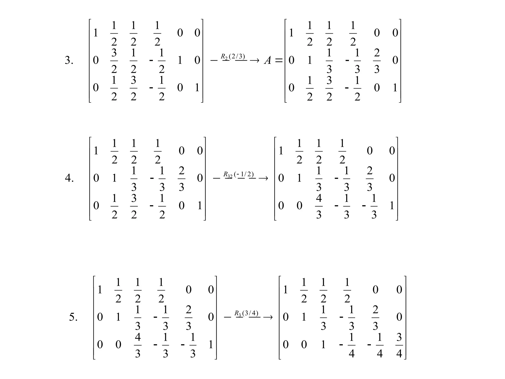
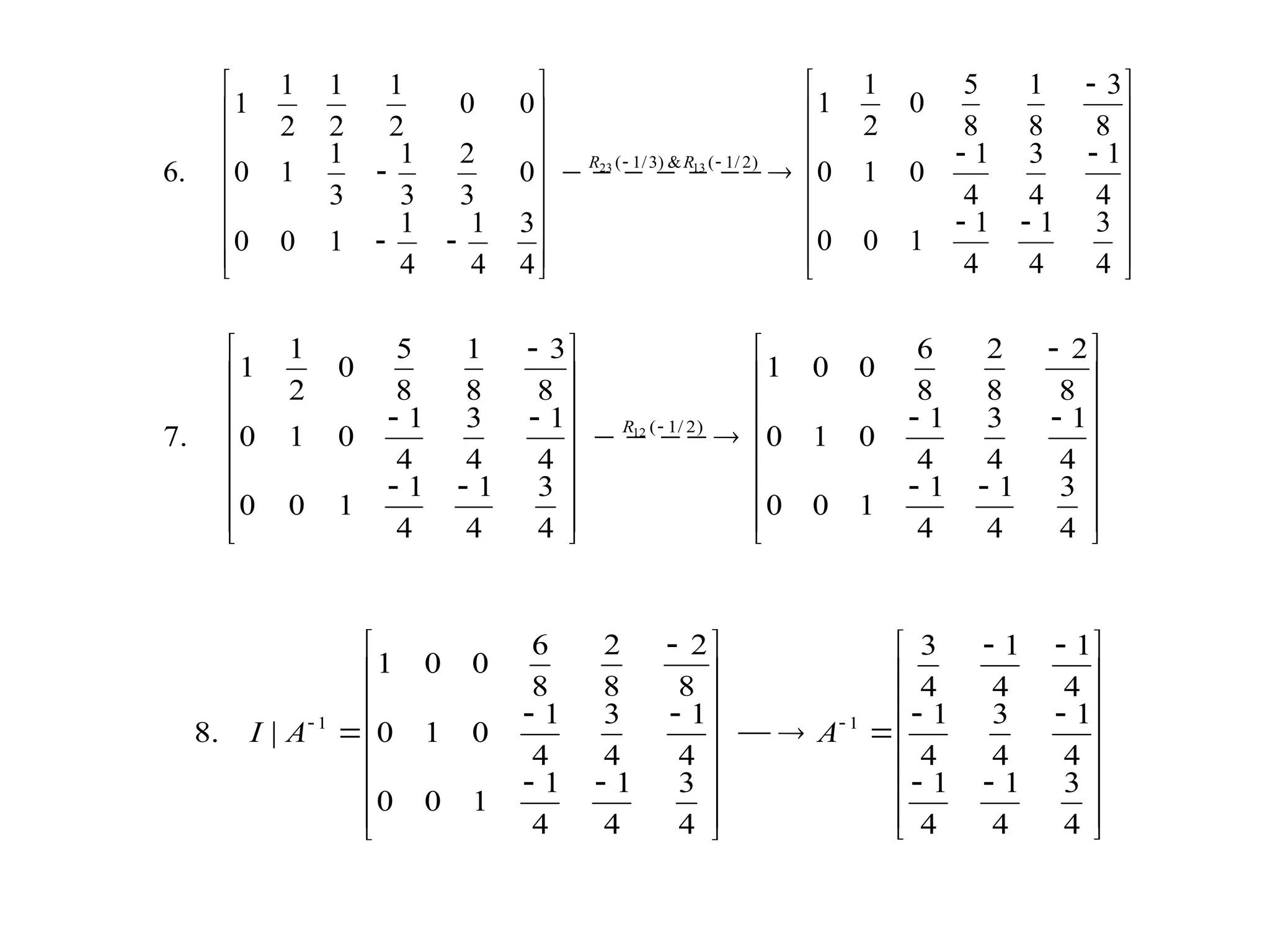
8. Gauss-Jordan Elimination: Example 2























 



























 























 
















 










































D
D
I
D
D
I
D
D
D
I
I
I
I
I
I
I
I
XX
YX
XY
XX
XX
YX
XY
XX
XX
R
R
XY
XX
YX
YY
XX
YX
XX
XY
XX
R
XX
YX
XY
XX
YX
YY
XX
XY
XX
R
R
YY
YX
XX
XY
XX
R
YY
YX
XY
XX
XY
XX
XY
XX
YX
YY
YX
XX
)
(
0
0
.
4
]
[
where
)
(
0
0
.
3
0
0
.
2
0
0
0
0
.
1
1
1
1
1
1
1
1
1
1
1
]
[
1
1
1
1
1
1
2
1
1
2
1
1
1
2
1
1
Partitioned inverse (using the Gauss-Jordan method).

9. Trace of a Matrix
 The trace of an n x n matrix A is defined to be the sum of the
elements on the main diagonal of A:
trace(A) = tr (A) = Σi aii.
where aii is the entry on the ith row and ith column of A.
 Properties:
- tr(A + B) = tr(A) + tr(B)
- tr(cA) = c tr(A)
- tr(AB) = tr(BA)
- tr(ABC) = tr(CAB) (invariant under cyclic
permutations.)
- tr(A) = tr(AT
)
- d tr(A) = tr(dA) (differential of trace)
- tr(A) = rank(A) when A is idempotent –i.e., A=
A2
.

10. Application: Rank of the Residual Maker
 We define M, the residual maker, as:
M = In - X(X′X)-1
X′ = In - P
where X is an nxk matrix, with rank(X)=k
 Let’s calculate the trace of M:
tr(M) = tr(In) - tr(P) = n - k
- tr(IT) = n
- tr(P) = k
Recall tr(ABC) = tr(CAB)
=> tr(P) = tr(X(X′X)-1
X′) = tr(X′X (X′X)-1
) = tr(Ik) = k
 Since M is an idempotent matrix –i.e., M= M2
-, then
rank(M) = tr(M) = n - k

11. Determinant of a Matrix
 The determinant is a number associated with any squared matrix.
 If A is an n x n matrix, the determinant is |A| or det(A).
 Determinants are used to characterize invertible matrices. A
matrix is invertible (non-singular) if and only if it has a non-zero
determinant
 That is, if |A|≠0 → A is invertible.
 Determinants are used to describe the solution to a system of
linear equations with Cramer's rule.
 Can be found using factorials, pivots, and cofactors! More on this
later.
 Lots of interpretations

12.  Used for inversion. Example: Inverse of a 2x2 matrix:







d
c
b
a
A bc
ad
A
A 

 )
det(
|
|











a
c
b
d
bc
ad
A
1
1 This matrix is called the
adjugate of A (or adj(A)).
A-1
= adj(A)/|A|

13. Determinant of a Matrix (3x3)
ceg
bdi
afh
cdh
bfg
aei
i
h
g
f
e
d
c
b
a






i
h
g
f
e
d
c
b
a
i
h
g
f
e
d
c
b
a
i
h
g
f
e
d
c
b
a Sarrus’ Rule: Sum from left to
right. Then, subtract from right
to left
Note: N! terms

14. Determinants: Properties
 Interchange of rows and columns does not affect |A|.
(Corollary, |A| = |A’|.)
 To any row (column) of A we can add any multiple of any
other row (column) without changing |A|.
 (Corollary, if we transform A into U or L , |A|=|U| = |L|,
which is equal to the product of the diagonal element of U or
L.)
 |I| = 1, where I is the identity matrix.
 |kA| = kn
|A|, where k is a scalar.
 |A| = |A’|.
 |AB| = |A||B|.
 |A-1
|=1/|A|.