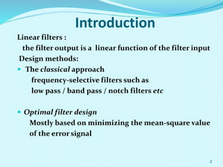
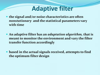
This document discusses linear filters and adaptive filters. It provides an overview of key concepts such as:
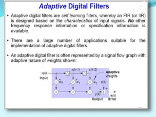
- Linear filters have outputs that are linear functions of their inputs, while adaptive filters can adjust their parameters over time based on the input signals.
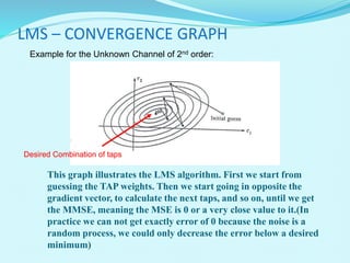
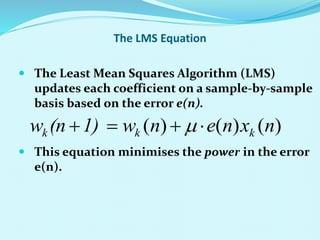
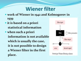
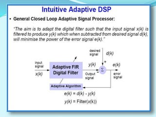
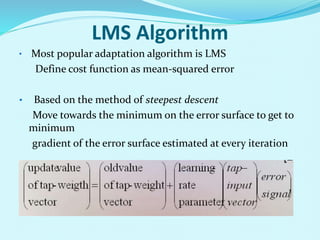
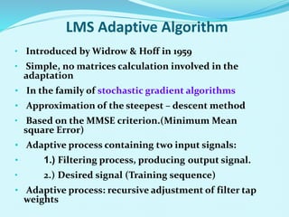
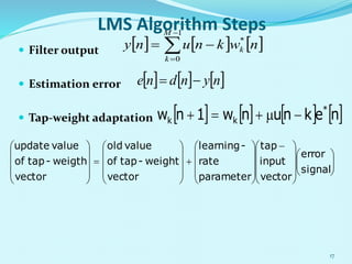
- The Wiener filter and LMS algorithm are introduced as approaches for optimal and adaptive filter design, with the LMS algorithm minimizing the mean square error using gradient descent.
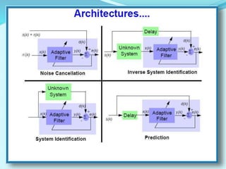
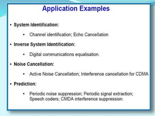
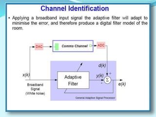
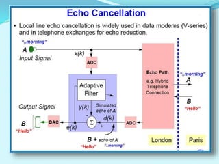
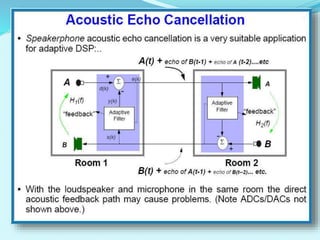
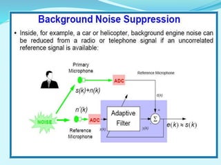
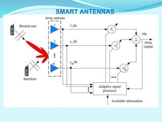
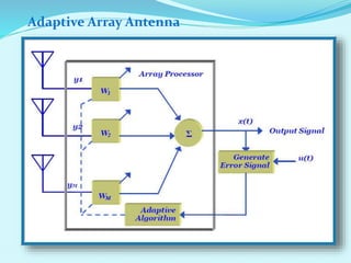
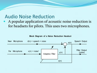
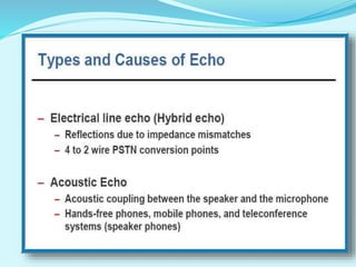
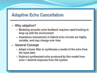
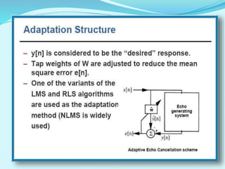
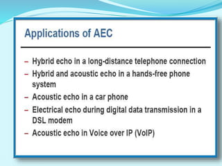
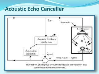
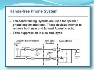
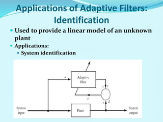
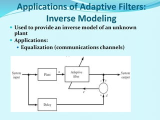
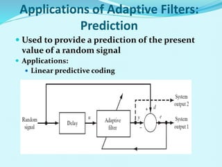
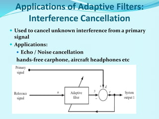
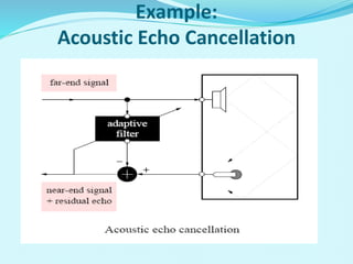
- Applications of adaptive filters include system identification, inverse modeling, prediction, and interference cancellation. An example of acoustic echo cancellation is described.
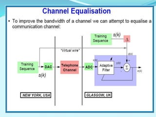
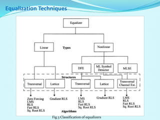
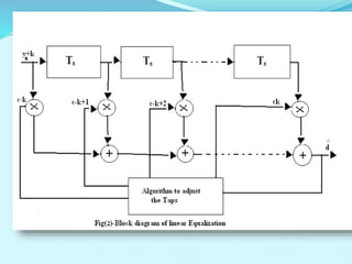
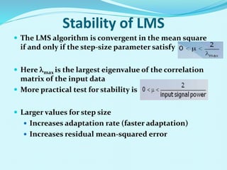
- The document outlines the LMS adaptive algorithm steps and discusses its stability and convergence properties. It also summarizes different equalization techniques for mitigating inter


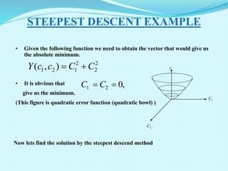
![• We start by assuming (C1 = 5, C2 = 7)
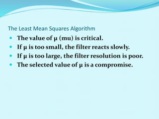
• We select the constant . If it is too big, we miss the minimum. If it is too
small, it would take us a lot of time to het the minimum. I would select =
0.1.
• The gradient vector is:
STEEPEST DESCENT EXAMPLE
]
[
2
1
]
[
2
1
]
[
2
1
]
[
2
1
]
1
[
2
1
9
.
0
1
.
0
2
.
0
n
n
n
n
n
C
C
C
C
C
C
y
C
C
C
C
2
1
2
1
2
2
C
C
dc
dy
dc
dy
y
• So our iterative equation is:](https://image.slidesharecdn.com/th-240123153739-85ee0024/85/Introduction-to-adaptive-filtering-and-its-applications-ppt-20-320.jpg)
![STEEPEST DESCENT EXAMPLE
567
.
0
405
.
0
:
3
3
.
6
5
.
4
:
2
7
5
:
1
2
1
2
1
2
1
C
C
Iteration
C
C
Iteration
C
C
Iteration
0
0
lim
013
.
0
01
.
0
:
60
......
]
[
2
1
2
1
n
n
C
C
C
C
Iteration
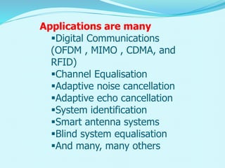
As we can see, the vector [c1,c2] converges to the value which would yield the
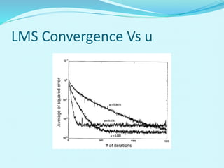
function minimum and the speed of this convergence depends on .
1
C
2
C
y
Initial guess
Minimum](https://image.slidesharecdn.com/th-240123153739-85ee0024/85/Introduction-to-adaptive-filtering-and-its-applications-ppt-21-320.jpg)