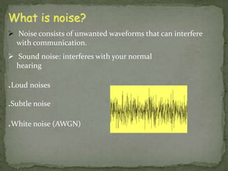
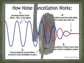
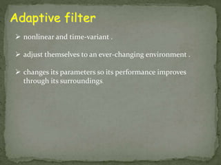
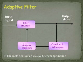
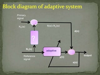
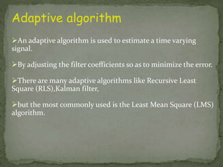
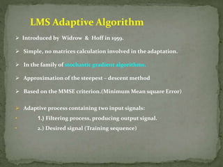
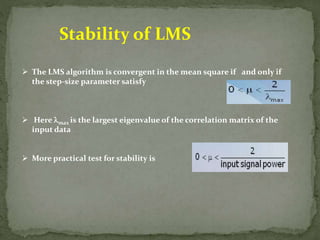
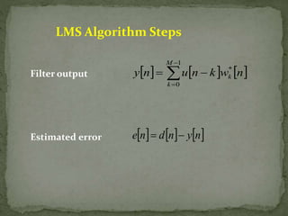
Done By 
S . Malki Hussain S.Chand Basha 
S . Md .Javeed B.Hussain Basha 
S.Baba Fakruddin S.Minuddin 
Submitted to 
S . Fouziya Parveen
 Goal 
 What is noise ? 
 What is Noise Cancellation ? 
 Simple Idea . 
 Applications 
 Adaptive Filter 
 Adaptive Algorithm( LMS ) 
 Simulation 
 Conclusion
Goal 
The goal of the project is for 
.
Equipment Lists 
Design Tools 
 MATLAB/Simulink 
 Xilinx System Generator
Design Approach 
Simulation 
 MATLAB 
. Least Mean Square (LMS) 
 Xilinx 
. Lease Mean Square (LMS)
What is noise? 
 Noise consists of unwanted waveforms that can interfere 
with communication. 
 Sound noise: interferes with your normal 
hearing 
.Loud noises 
.Subtle noise 
.White noise (AWGN)
What is Noise Cancellation? 
 Noise cancellation is a method to reduce or completely cancel out 
undesirable sound. 
 call Active Noise Cancellation . 
 Noise cancellation tries to 'block' the sound at the source instead of 
trying to prevent the sounds from entering our ear canals . 
 These technologies are in their early stages. 
 The hope is that one day that these technologies can be used to 
minimize all sorts of unwanted sounds around us
Simple Idea 
 Cancellation processes depend on simple principle 
 adding two signals with the same 
 amplitude and opposite phase the result will be zero 
signals. 
(H)
Simple wave cancellation
Applications 
Headsets (headphone) 
Honda cars. 
Space satellite antennas. 
 Use in apartment. 
 Noise Muter
Adaptive Noise Cancelling 
 Adaptive noise cancelling 
- An approach to reduce noise based on reference noise 
signals 
- System output 
- The LMS algorithm 
K 
k 
  
u t s t n t w k n t k 
( )  ( )  ( )  ( ) (  
) 
0 1 1 ( ) ( ) ( ) 1 w k u t n t  k
Adaptive filter 
 nonlinear and time-variant . 
 adjust themselves to an ever-changing environment . 
 changes its parameters so its performance improves 
through its surroundings.
Adaptive Filter 
Output 
signal 
Input 
signal 
Adaptive 
algorithm 
Criterion of 
performance 
Filter 
structure 
 The coefficients of an adaptive filter change in time
Block diagram of adaptive system 
No(n) S(n)+No(n) 
? 
Primary 
signal 
d(n) 
N1(n) 
Reference 
signal 
y(n) 
output 
e(n) 
adaptive
Adaptive algorithm 
An adaptive algorithm is used to estimate a time varying 
signal. 
By adjusting the filter coefficients so as to minimize the error. 
There are many adaptive algorithms like Recursive Least 
Square (RLS),Kalman filter, 
but the most commonly used is the Least Mean Square (LMS) 
algorithm.
LMS Adaptive Algorithm 
 Introduced by Widrow & Hoff in 1959. 
 Simple, no matrices calculation involved in the adaptation. 
 In the family of stochastic gradient algorithms. 
 Approximation of the steepest – descent method 
 Based on the MMSE criterion.(Minimum Mean square Error) 
 Adaptive process containing two input signals: 
• 1.) Filtering process, producing output signal. 
• 2.) Desired signal (Training sequence)
Stability of LMS 
 The LMS algorithm is convergent in the mean square if and only if 
the step-size parameter satisfy 
 Here max is the largest eigenvalue of the correlation matrix of the 
input data 
 More practical test for stability is
LMS Algorithm Steps 
Filter output 
Estimated error 
 
       
y n  u n  
k w n 
k  
1 
0 
* 
M 
k 
en dn yn
The LMS Equation 
 The Least Mean Squares Algorithm (LMS) updates each coefficient 
on a sample-by-sample basis based on the error e(n). 
w (n 1) ( ) ( ) ( ) k w n e n x n k k     
 This equation minimises the power in the error e(n). 
 The value of μ (mu) is critical. 
 If μ is too small, the filter reacts slowly. 
 If μ is too large, the filter resolution is poor. 
 The selected value of μ is a compromise.
LMS algorithm 
 Estimates the 
solution to the 
Widrow -Hoff 
equations using gradient 
descent method which 
Finds minima by 
estimating 
the gradient. 
X(n) 
Transversal 
Filter 
C(n) 
LMS 
Y(n) 
d(n) 
e(n) 
is the step size
Cont.. 
e(n) 
Adaptive 
filter 
Unknown 
system 
X(n) 
y(n) 
d(n) 
filtering operation with the 
previous version of the coefficients. 
Compare the computed output 
with the expected output. 
Update the coefficients using 
the following computation.
Cont.. 
LMS algorithm 
The most widely used real time adaptive filtering algorithm 
Convergence speed of the LMS algorithm 
 Controlled by the spread of eigenvalues of the autocorrelation 
matrix of the input data 
 Enhanced by reducing the eigenvalue spread
Advantages 
 low computational complexity 
 simple to implement 
 allow real-time operation
Simulation 
Xilinx System Generator Output
Conclusion 
 Active noise cancellation is a method to cancel out 
undesirable sound in real time 
 The adaptive filter is used to estimate the error in 
noisy wave 
 Many algorithms are used in adaptive filter like LMS 
RLS & MSE and the better is LMS .
Low power vlsi implementation adaptive noise cancellor based on least means square algorithm

Low power vlsi implementation adaptive noise cancellor based on least means square algorithm

  • 1.
    Done By S. Malki Hussain S.Chand Basha S . Md .Javeed B.Hussain Basha S.Baba Fakruddin S.Minuddin Submitted to S . Fouziya Parveen
  • 2.
     Goal What is noise ?  What is Noise Cancellation ?  Simple Idea .  Applications  Adaptive Filter  Adaptive Algorithm( LMS )  Simulation  Conclusion
  • 3.
    Goal The goalof the project is for .
  • 4.
    Equipment Lists DesignTools  MATLAB/Simulink  Xilinx System Generator
  • 5.
    Design Approach Simulation  MATLAB . Least Mean Square (LMS)  Xilinx . Lease Mean Square (LMS)
  • 6.
    What is noise?  Noise consists of unwanted waveforms that can interfere with communication.  Sound noise: interferes with your normal hearing .Loud noises .Subtle noise .White noise (AWGN)
  • 7.
    What is NoiseCancellation?  Noise cancellation is a method to reduce or completely cancel out undesirable sound.  call Active Noise Cancellation .  Noise cancellation tries to 'block' the sound at the source instead of trying to prevent the sounds from entering our ear canals .  These technologies are in their early stages.  The hope is that one day that these technologies can be used to minimize all sorts of unwanted sounds around us
  • 8.
    Simple Idea Cancellation processes depend on simple principle  adding two signals with the same  amplitude and opposite phase the result will be zero signals. (H)
  • 9.
  • 10.
    Applications Headsets (headphone) Honda cars. Space satellite antennas.  Use in apartment.  Noise Muter
  • 11.
    Adaptive Noise Cancelling  Adaptive noise cancelling - An approach to reduce noise based on reference noise signals - System output - The LMS algorithm K k   u t s t n t w k n t k ( )  ( )  ( )  ( ) (  ) 0 1 1 ( ) ( ) ( ) 1 w k u t n t  k
  • 13.
    Adaptive filter nonlinear and time-variant .  adjust themselves to an ever-changing environment .  changes its parameters so its performance improves through its surroundings.
  • 14.
    Adaptive Filter Output signal Input signal Adaptive algorithm Criterion of performance Filter structure  The coefficients of an adaptive filter change in time
  • 15.
    Block diagram ofadaptive system No(n) S(n)+No(n) ? Primary signal d(n) N1(n) Reference signal y(n) output e(n) adaptive
  • 16.
    Adaptive algorithm Anadaptive algorithm is used to estimate a time varying signal. By adjusting the filter coefficients so as to minimize the error. There are many adaptive algorithms like Recursive Least Square (RLS),Kalman filter, but the most commonly used is the Least Mean Square (LMS) algorithm.
  • 17.
    LMS Adaptive Algorithm  Introduced by Widrow & Hoff in 1959.  Simple, no matrices calculation involved in the adaptation.  In the family of stochastic gradient algorithms.  Approximation of the steepest – descent method  Based on the MMSE criterion.(Minimum Mean square Error)  Adaptive process containing two input signals: • 1.) Filtering process, producing output signal. • 2.) Desired signal (Training sequence)
  • 18.
    Stability of LMS  The LMS algorithm is convergent in the mean square if and only if the step-size parameter satisfy  Here max is the largest eigenvalue of the correlation matrix of the input data  More practical test for stability is
  • 19.
    LMS Algorithm Steps Filter output Estimated error         y n  u n  k w n k  1 0 * M k en dn yn
  • 20.
    The LMS Equation  The Least Mean Squares Algorithm (LMS) updates each coefficient on a sample-by-sample basis based on the error e(n). w (n 1) ( ) ( ) ( ) k w n e n x n k k      This equation minimises the power in the error e(n).  The value of μ (mu) is critical.  If μ is too small, the filter reacts slowly.  If μ is too large, the filter resolution is poor.  The selected value of μ is a compromise.
  • 21.
    LMS algorithm Estimates the solution to the Widrow -Hoff equations using gradient descent method which Finds minima by estimating the gradient. X(n) Transversal Filter C(n) LMS Y(n) d(n) e(n) is the step size
  • 22.
    Cont.. e(n) Adaptive filter Unknown system X(n) y(n) d(n) filtering operation with the previous version of the coefficients. Compare the computed output with the expected output. Update the coefficients using the following computation.
  • 23.
    Cont.. LMS algorithm The most widely used real time adaptive filtering algorithm Convergence speed of the LMS algorithm  Controlled by the spread of eigenvalues of the autocorrelation matrix of the input data  Enhanced by reducing the eigenvalue spread
  • 24.
    Advantages  lowcomputational complexity  simple to implement  allow real-time operation
  • 26.
    Simulation Xilinx SystemGenerator Output
  • 27.
    Conclusion  Activenoise cancellation is a method to cancel out undesirable sound in real time  The adaptive filter is used to estimate the error in noisy wave  Many algorithms are used in adaptive filter like LMS RLS & MSE and the better is LMS .