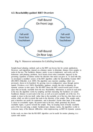
This document describes a motion planning algorithm for bounding locomotion of the LittleDog robot over rough terrain. It presents a planar five-link model of LittleDog with a 16-dimensional state space. A modified rapidly exploring random tree (RRT) algorithm is used to efficiently find feasible motion plans that respect the robot's kinodynamic constraints. The algorithm incorporates motion primitives, reachability guidance to address differential constraints, and sampling in a lower-dimensional task space. Feedback control based on transverse linearization is also implemented to stabilize planned trajectories in simulation and experiments. Open-loop bounding is inherently unstable, so feedback control is needed for reliable dynamic locomotion.

1. Index
Abstract.............................................................................................01
1. Introduction..................................................................................01
2. Background...................................................................................03
2.1. Planning Approaches................................................................03
2.2. Limit-cycle Approach................................................................05
2.3. Dynamic Maneuvers..................................................................05
3. LittleDog Model............................................................................05
3.1. Motor Model...............................................................................07
3.2. Ground Interaction Model........................................................08
3.3. Parameter Estimation...............................................................09
3.4. Model Performance...................................................................09
4. Motion Planning Algorithm.........................................................11
4.1. Problem Formulation.................................................................................11
4.2. Macro Actions/Motion Primitive.............................................12
4.3. Reachability-guided RRT Overview........................................13
4.4. Approximating the Reachable Set............................................14
4.5. Sampling in Task Space............................................................15
4.6. Simulation Results.....................................................................15
4.7. Experimental Results.................................................................15
5. Feedback Stabilization.................................................................15
5.1. Selection of Projection and Optimization Weights.................16
5.2. Simulation Results.....................................................................16
5.3. Experimental Results.................................................................16
6. Concluding Remarks and Future Directions.............................16
7 Acknowledgements........................................................................17
8 References.......................................................................................17

2. Robotics
Abstract
A motion planning algorithm is described for bounding over rough terrain with the LittleDog
robot. Unlike walking gaits, bounding is highly dynamic and cannot be planned with quasi-
steady approximations. LittleDog is modeled as a planar five-link system, with a 16-
dimensional state space; computing a plan over rough terrain in this high-dimensional state
space that respects the kinodynamic constraints due to underactuation and motor limits is
extremely challenging. Rapidly Exploring Random Trees (RRTs) are known for fast
kinematic path planning in high-dimensional configuration spaces in the presence of
obstacles, but search efficiency degrades rapidly with the addition of challenging dynamics.
A computationally tractable planner for bounding was developed by modifying the RRT
algorithm by using: (1) motion primitives to reduce the dimensionality of the problem; (2)
Reachability Guidance, which dynamically changes the sampling distribution and distance
metric to address differential constraints and discontinuous motion primitive dynamics; and
(3) sampling with a Voronoi bias in a lower-dimensional “task space” for bounding. Short
trajectories were demonstrated to work on the robot, however open-loop bounding is
inherently unstable. A feedback controller based on transverse linearization was
implemented, and shown in simulation to stabilize perturbations in the presence of noise and
time delays.
1. Introduction
While many successful approaches to dynamic legged locomotion exist, we do not yet have
approaches which are general and flexible enough to cope with the incredible variety of
terrain traversed by animals. Progress in motion planning algorithms has enabled general and
flexible solutions for slowly moving robots, but we believe that in order to quickly and
efficiently traverse very difficult terrain, extending these algorithms to dynamic gaits is
essential. In this work we present progress towards achieving agile locomotion over rough
terrain using the LittleDog robot. LittleDog (Figure 1) is a small, 3-kg position-controlled
quadruped robot with point feet and was developed by Boston Dynamics under the DARPA
Learning Locomotion program. The program ran over several phases from 2006 to 2009, and
challenged six teams from universities around the United States to compete in developing
algorithms that enable LittleDog to navigate known, uneven terrain, as quickly as possible.
The program was very successful, with many teams demonstrating robust planning and
locomotion over quite challenging terrain (e.g. Pongas et al. 2007; Rebula et al. 2007; Kolter
et al. 2008; Zucker 2009), with an emphasis on walking gaits, and some short .

3. Achieving bounding on LittleDog is difficult for a number of reasons. First, the robot is
mechanically limited:
high-gear ratio transmissions generally provide sufficient torque but severely limit joint
velocities and complicate any attempts at direct torque control. Second, a stiff frame
complicates impact modeling and provides essentially no opportunity for energy storage.
Finally, and more generally, the robot is underactuated, with the dynamics of the unactuated
joints resulting in a complicated dynamical relationship between the actuated joints and the
interactions with the ground. These effects are dominant enough that they must be considered
during the planning phase.
In this work, we propose a modified form of the Rapidly Exploring Random Tree (RRT)
(LaValle and Kuffner 2001) planning framework to quickly find feasible motion plans for
bounding over rough terrain. The principal advantage of the RRT is that it respects the
kinematic and dynamic constraints which exist in the system, however for high-dimensional
robots the planning can be prohibitively
slow. We highlight new sampling approaches that improve the RRT efficiency. The
dimensionality of the system is addressed by biasing the search in a low-dimensional task
space. A second strategy uses reachability guidance as a heuristic to encourage the RRT to
explore in directions that are most likely to successfully expand the tree into previously
unexplored regions of state space. This allows the RRT to incorporate smooth motion
primitives, and quickly find plans despite challenging differential constraints introduced by
the robot’s underactuated dynamics. This planner operates on a carefully designed model of
the robot dynamics which includes the subtleties of motor saturations and ground
interactions.
Bounding motions over rough terrain are typically not stable in open loop: small
disturbances away from the nominal trajectory or inaccuracies in physical parameters used
for planning can cause the robot to fall over. To achieve reliable bounding it is essential to
design a feedback controller to robustly stabilize the planned motion. This stabilization
problem is challenging due to the severe underactuation of the robot and the highly dynamic
nature of the planned trajectories. We implemented a feedback controller based on the

4. method of transverse linearization which has recently emerged as an enabling technology for
this type of control problem (Hauser and Chung 1994; Shiriaev et al. 2008; Manchester et al.
2009; Manchester 2010).
The remainder of this paper is organized as follows: in Section 2 we begin by
reviewing background information, including alternative approaches to achieve legged
locomotion over rough terrain with particular attention given to motion planning approaches.
In Section 3 we present a comprehensive physics-based model of the LittleDog robot and the
estimation of its parameters from experiments. Section 4 discusses motion planning for bounding,
with a detailed description of the technical approach and experimental results. In Section 5,
we describe the feedback control design and show some simulation and experimental results.
2. Background
The problem of fast locomotion over rough terrain has been an active research topic in
robotics, beginning with the seminal work by Raibert in the 1980s (Raibert 1986; Raibert et
al. 1986). The research can be roughly divided into two categories. The first category uses
knowledge of the robot and environment within a motion planning framework. This approach
is capable of versatile behavior over rough terrain, but motion plans tend to be slow and
conservative. The other category is characterized by a limit-cycle approach, which is usually
blind to the environment. In this approach, more dynamic motions may be considered, but
typically over only a limited range of behavior. In this section we review these approaches in
turn.
2.1. Planning Approaches
Planning algorithms have made significant headway in recent years. These methods are
particularly well developed for kinematic path planning in configuration space, focusing on
maneuvers requiring dexterity, obstacle avoidance, and static stability. Sampling-based
methods such as the RRT are very effective in planning in high-dimensional humanoid
configuration spaces. The RRT has been used to plan walking and grasping trajectories
amidst obstacles by searching for a collision-free path in configuration space, while
constraining configurations to those that are statically stable (Kuffner et al. 2002, 2003). The
robot is statically stable when the center of mass (COM) is directly above the support
polygon, therefore guaranteeing that the robot will not roll over as long as the motion is
executed slowly enough. After finding a statically feasible trajectory of configurations
(initially ignoring velocity), the trajectory is locally optimized for speed and smoothness,
while maintaining the constraint that at least one foot remains flat on the ground at all times.
This approach
has been extended to account for moving obstacles and demonstrated on the Honda Asimo
(Chestnutt et al. 2005). An alternative approach is to first generate a walking pattern while
ignoring obstacles and collisions, and then use random sampling to modify the gait to avoid
obstacles while verifying constraints to ensure the robot does not fall (Harada et al. 2007).
Current methods are adept at planning in high-dimensional configuration spaces, but typically
only for limited dynamic motions. Sampling-based planning algorithms are in general not
well suited for planning fast dynamic motions, which are governed largely by underactuated
dynamics.

5. The use of static stability for planning allows one to ignore velocities, which halves the size
of the state space,
and constrains the system to be fully actuated, which greatly simplifies the planning problem.
Statically stable motions are, however, inherently conservative (technically a robot is truly
statically stable only when it is not moving). This constraint can be relaxed by using a
dynamic stability criteria (see Pratt and Tedrake (2005) for review of various metrics). These
metrics can be used either for gait generation by the motion planner, or as part of a feedback
control strategy. One popular stability metric requires the center of pressure, or the Zero
Moment Point (ZMP), to be within the support polygon defined by the convex hull of the feet
contacts on the ground. While the ZMP is regulated to remain within the support polygon, the
robot is guaranteed not to roll over any edge of the support polygon. In this case, the
remaining degrees of freedom can be controlled as if the system is
fully actuated using standard feedback control techniques applied to fully actuated systems.
Such approaches have been successfully demonstrated for gait generation and execution on
humanoid platforms such as the Honda Asimo (Sakagami et al. 2002; Hirose and Ogawa
2007), and the HRP series of walking robots (Kaneko et al. 2004). Lowerdimensional
“lumped” models of the robot can be used to simplify the differential equations that define
ZMP. In Kajita et al. (2003), the HRP-2 robot was modeled as a cart (rolling point mass) on
top of a table (with a small base that should not roll over). Preview control was then applied
to generate a COM trajectory which regulates the desired ZMP position. Note that although
the ZMP is only defined on flat terrain, some extensions can be applied to extend the idea to
3D, including using hand contacts for stability, for example by considering the Contact
Wrench Sum (CWS) (Sugihara 2004).
The works described so far were mostly demonstrated on relatively flat terrain. Other quasi-
static planning
approaches were applied to enable climbing behaviour and walking over varied terrain with
the HRP-2 humanoid robot (Hauser et al. 2008; Hauser 2008). In that work, contact points
and equilibrium (static) stances, acting as way points, were chosen by using a Probabilistic
Road Map (Kavraki et al. 1996), an alternative sampling-based planning strategy. The
planner searched for paths through potentially feasible footholds and stances, while taking
into account contact and equilibrium constraints to ensure that the robot maintains a foot or
hand hold, and does not slip. Motion primitives were then used to find quasi-static local
motion plans between stances that maintain the non-slip constraints. With a similar goal of
traversing very rough terrain with legged robots, the DARPA Learning Locomotion project,
utilizing the LittleDog robot, has pushed the envelope of walking control by using careful
foot placement. Much of the work developed in this program has combined path planning and
motion primitives to enable crawling gaits on rough terrain (e.g. Pongas et al. 2007;
Rebula et al. 2007; Kolter et al. 2008; Ratliff et al. 2009). Similar to the approaches of the
other teams, during the first two phases of the program, MIT utilized heuristics over the
terrain to assign a cost to potential footholds. A* search was then used to find a trajectory of
feasible stances over the lowest cost footholds, and a ZMP-based body motion and swing-
foot motion planner was used to generate trajectories
to walk over rough terrain. Use of stability metrics such as ZMP have advanced the state of
the art in planning gaits over rough terrain, however these stability constraints result in very
conservative dynamic trajectories, for example by requiring that at least one foot is always
flat on the ground. Because ZMP-based control systems do not reason about underactuated
dynamics, the humanoid robots do not perform well when walking on very rough or
unmodeled terrain, cannot move nearly as quickly as humans, and use dramatically more

6. energy (appropriately scaled) than a human (Collins et al. 2005). Animals do not constrain
themselves to such a regime of operation. Much more agile behavior takes place precisely
when the system is operating in an underactuated regime, for example during an aerial phase,
or while rolling the foot over the toe while walking. In such regimes, there is no support
polygon, so the legged robot is essentially falling and catching itself. Furthermore,
underactuated dynamics might otherwise be exploited: for example, a humanoid
robot can walk faster and with longer strides by rolling the foot over the toe.
2.2. Limit-cycle Approach
Somewhat orthogonal to the planning approaches, a significant body of research focuses on
limit-cycle analysis for walking. Tools developed for limit-cycle analysis allow one to
characterize the behavior of a particular gait, typically on flat terrain. Stable limit-cycle
locomotion can be achieved by using compliant or mechanically clever designs that enable
passive stability using open-loop gaits (e.g. Collins et al. 2005), or otherwise through the use
of reflexive control algorithms that tend to react to terrain. Recent applications of these
strategies, for example on the Rhex robot (Altendorfer et al. 2001) and BigDog (Raibert et al.
2008), have produced impressive results, but these systems do not take into account
knowledge about upcoming terrain. Feedback control of underactuated “dynamic walking”
bipeds has recently been approached using a variety of
control methods, including virtual holonomic constraints (Chevallereau et al.
2003;Westervelt et al. 2003, 2007) with which impressive results have been demonstrated for
a single limit-cycle gait over flat terrain. In this paper, we use an alternative method based on
the combination of transverse linearization and time-varying linear control techniques
(Shiriaev et al. 2008; Manchester et al. 2009; Manchester 2010). This allows one to stabilize
more general motions, however a nominal trajectory is required in advance, so this feedback
controller must be paired with a motion planning algorithm which takes into account
information about the environment.
2.3. Dynamic Maneuvers
In order to use sample-based planning for a highly dynamic, underactuated robot, the search
must take place in the complete state space, as velocities play an important role in the
dynamics. This effectively doubles the dimension of the search. Furthermore, when there are
underactuated dynamics, the robot cannot accelerate in arbitrary directions, and therefore can
only move in state space in very limited directions. This makes straightforward application of
samplebased planning extremely challenging for these types of systems. In the second phase
of the LittleDog program, our team began to integrate dynamic lunging, to move two feet
at a time (Byl et al. 2008; Byl and Tedrake 2009), into the otherwise quasi-static motion plans
to achieve fast locomotion over rough terrain. This paper describes the MIT team approach in
the third (final) phase of the project. We show that careful foot placement can be combined
with highly dynamic model-based motion planning and feedback control to achieve
continuous bounding over very rough terrain.
3. LittleDog Model
An essential component of any model-based planning approach is a sufficiently accurate
identification of the system dynamics. Obtaining an accurate dynamic model for LittleDog is
challenging owing to subtleties in the ground interactions and the dominant effects of motor

7. saturations and transmission dynamics. These effects are more pronounced in bounding gaits
than in walking gaits, due to the increased magnitude of ground reaction forces at impact and
the perpetual saturations of the motor; as a result, we required a more detailed model. In this
section, we describe our system identification procedure and results.
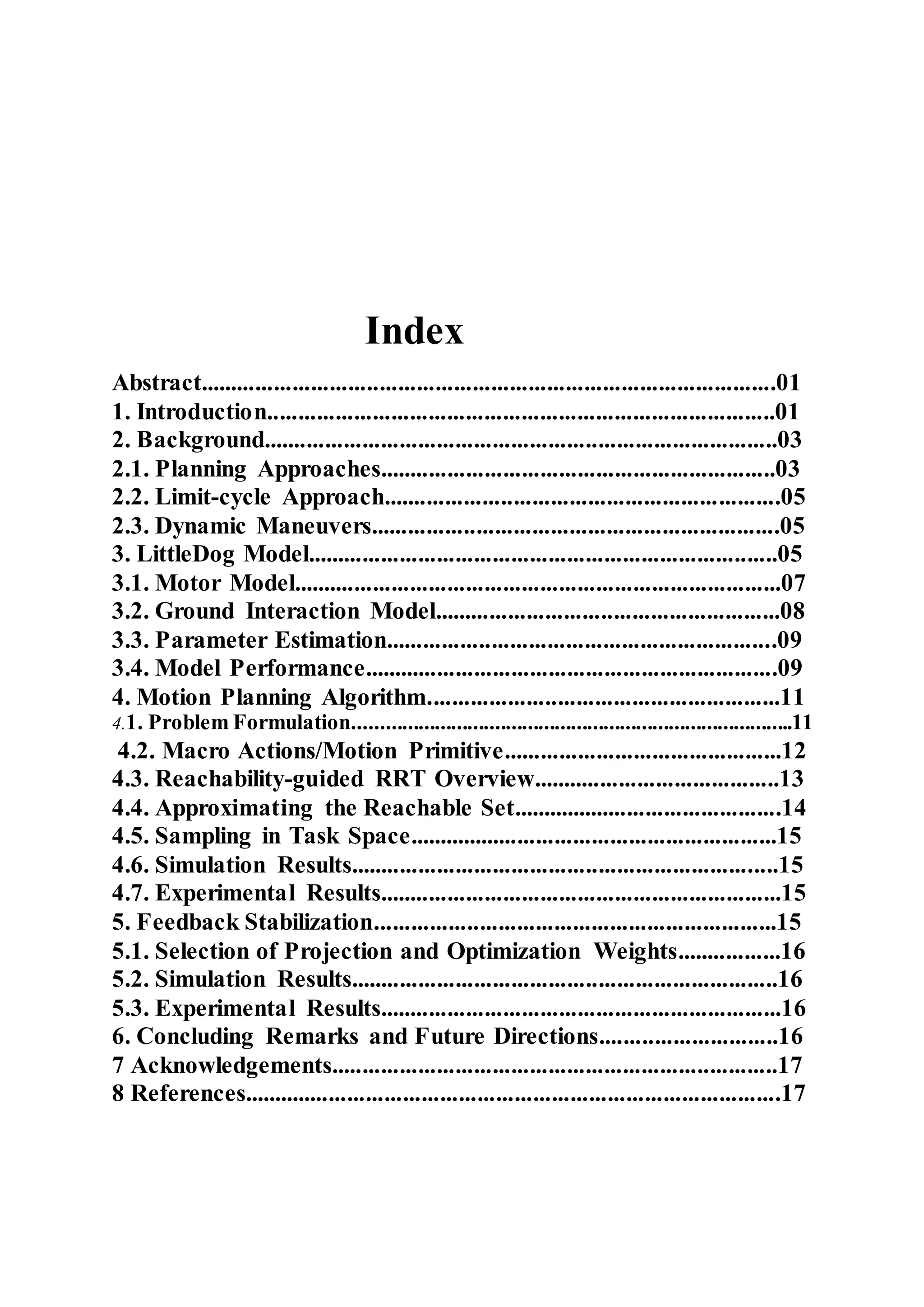
The LittleDog robot has 12 actuators (two in each hip, one in each knee) and a total of 22
essential degrees of
freedom (six for the body, three rotational joints in each leg, and one prismatic spring in each
leg). By assuming that the leg springs are over-damped, yielding first-order dynamics, we
arrive at a 40-dimensional state space (18 × 2 + 4). However, to keep the model as simple
(low-dimensional) as possible, we approximate the dynamics of the robot using a planar five-
link serial rigid-body chain model, with revolute joints connecting the links, and a free base
joint, as shown in Figure 3. The planar model assumes that the back legs move together as
one and the front legs move together as one (see Figure 1). Each leg has a single hip joint,
connecting
the leg to the main body, and a knee joint. The foot of the real robot is a rubber-coated ball
that connects to the
shin through a small spring (force sensor), which is constrained to move along the axis of the
shin. The spring is
stiff, heavily damped, and has a limited travel range, so it is not considered when computing
the kinematics of the robot, but is important for computing the ground forces. In addition, to
reduce the state space, only the length of the shin spring is considered. This topic s discussed
in detail as part
of the ground contact model.
The model’s seven-dimensional configuration space, C = R2 × T5, consists of the planar
position of the back foot( x, y), the pitch angle ω, and the 4 actuated joint angles q1, . . . , q4.
The full state of the robot, x = [q, ˙q, l] ∈ X, has 16 dimensions and consists of the robot
configuration, the corresponding velocities, and the two prismatic shin-spring lengths, l = [l1,
l2], one for each foot. The control command, u, specifies reference angles for the four
actuated joints. The robot receives joint commands at 100 Hz and then applies an internal PD
controller at 500 Hz. For simulation, planning and control purposes, the dynamics are defined
as
x[n + 1] = f ( x[n], u[n]) , (1)
where x[n+1] is the state at t[n+1], x[n] is the state at t[n], and u[n] is the actuated joint
position command applied during the time interval between t[n] and t[n+1].We sometimes
refer to the control time step, _T = t[n+1]−t[n] = 0.01 seconds. A fixed-step fourth-order
Runge–Kutta integration of the continuous Euler–Lagrange dynamics model is used to
compute the state update.
A self-contained motor model is used to describe the movement of the actuated joints.
Motions of these joints
are prescribed in the five-link system, so that as the dynamics are integrated forward, joint
torques are back-computed, and the joint trajectory specified by the model is exactly
followed. This model is also constrained so that actuated joints respect bounds placed on
angle limits, actuator velocity limits, and actuator torque limits. In addition, forces computed
from a ground contact model are applied to the five-link chain when the feet are in contact
with the ground. The motor model and ground contact forces are described in more detail
below. The actuated joints are relatively stiff, so the model is most important for predicting

8. the motion of the unactuated degrees of freedom of the system, in particular the pitch angle,
as well as the horizontal position of the robot.
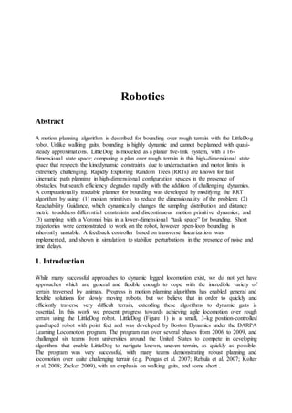
3.1. Motor Model
The motors on LittleDog have gear ratios of approximately 70 : 1. Because of the high gear
ratio, the internal secondorder dynamics of the individual motors dominate in most cases, and
the rigid-body dynamics of a given joint, as well as effects of inertial coupling and external
forces on the robot can be neglected. The combination of the motor internal dynamics with
the PD controller with fixed PD gains can be accurately modeled as a linear second-order
system:
q¨i = −bq˙i + k( ui − qi) , (2)
where q¨i is the acceleration applied to the ith joint, giventhe state variables [qi, q˙i] and the
desired position ui. To account for the physical limitations of actual motors, the model
includes hard saturations on the velocity and acceleration of the joints. The velocity limits, in
particular, have a large effect on the joint dynamics.
Each of the four actuated joints is assumed to be controlled by a single motor, with both of
the knee joints having one pair of identical motors, and the hip joints having a different pair
of identical motors (the real robot has different echanics in the hip versus the knee). Owing to
this, two separate motor parameter sets: {b, k, vlim, alim} are used, one for the knees, and
one for the hips.
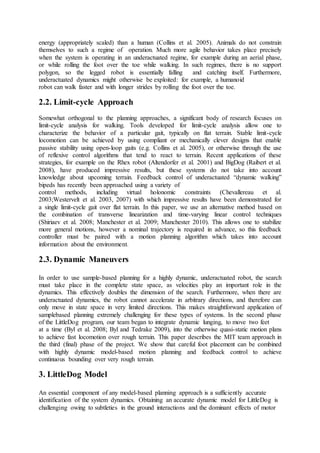
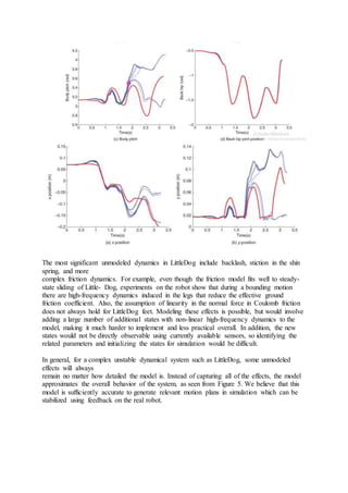
Figure 4 shows a typical fit of the motor model to real trajectories. The fits are consistent
across the different joints of the robot and across different LittleDog robots, but depend on
the gains of the PD controller at each of the joints. As seen from the figure, the motor model
does well in tracking the actual joint position and velocity. Under large dynamic loads, such
as when the hip is lifting and accelerating the whole robot body at the beginning of a bound,
the model might slightly lead the actual joint readings. This can be seen in Figure 4 (top) at
5.4 s. For the knee joint and for less aggressive trajectories with the hip, the separation is not
significant. In addition, note that backlash in the joints is not modeled. The joint encoders or

9. located on the motors rather than the joint axes, which makes it very difficult to measure and
model backlash.
3.2. Ground Interaction Model
LittleDog is mostly incapable of an aerial phase due to the velocity limits in the joints, so at
least one foot is usually in contact with the ground at any time. The ground interaction is
complicated, because the robot’s foot may roll, slide, stick, bounce, or do some combination
of these. A continuous, elastic ground interaction model is used, where the foot of the robot is
considered as a ball, and at each point in time the forces acting on the foot are computed. The
ground plane is assumed to be compressible, with a stiff non-linear spring damper normal to
the ground that pushes the foot out of the terrain. A tangential friction force, based on a non-
linear model of Coulomb friction is also assumed. The normal and friction forces are
balanced with the force of the shin spring at the bottom of the robot’s leg. The rate of change
of the shin spring, ˙l, is computed by the force balancing and used to update the shin-spring
length, l, which is a part of the state space. The resulting normal and friction forces are
applied to the five-link model.
Appendix A discusses the details of the foot roll calculation, the normal force model, the
friction model, and their use in computing ground contact forces. The ground contact model
is also illustrated in Figure 21 of the Appendix.

10. 3.3. Parameter Estimation
There are many coupled parameters that determine the behavior of the model. In theory, they
could all be fit
to a large enough number of robot trajectories, but it would require thoroughly exploring
relevant regions of the
robot’s {STATE-SPACE × ACTION-SPACE}. This is difficult, because LittleDog cannot
easily be set to an arbitrary point in state space, and the data we collect only covers a tiny
fraction of it. An easier and more robust approach relies on the model structure to separate
the fitting into sub-problems and to identify each piece separately. The full dynamical model
of the robot consists of the five-link rigid body,
the motor model, and the ground force model. A series of experiments and a variety of short
bounding trajectories were used to fit the model parameters to actual robot dynamics by
minimizing quadratic cost functions over simulation error. Appendix B discusses the
approach for the fit and lists the parameters and their values. In total, 34 parameters were
measured or fit for the model.
3.4. Model Performance
Figure 5 shows a comparison of a bounding trajectory in simulation versus 10 runs of the
same command executed on the real robot. The simulated trajectory was generated using the
planning algorithm described in the next section, which used the developed model. The
control input and the starting conditions for all open-loop trajectories in the figure were
identical, and these trajectories were not used for fitting the model parameters. Three of the
four plots are of an unactuated coordinate (x, y, and body pitch), the fourth plot is of the back
hip, an actuated joint. The figure emphasizes the difference between directly actuated,
position controlled joints compared with unstable and unactuated degrees of freedom. While
the motor model tracks the joint positions almost perfectly, even through collisions with the
ground, the unactuated coordinates of the open-loop trajectories diverge from each other in
less than 2 seconds. Right after complet the first bounding motion, at about 1.5 s, the
trajectories separate as LittleDog is lifting its body on the back feet. At about 1.9 s, in half of
the cases the robot falls forward and goes through a second bounding motion, while in the
rest of the cases it falls backward and cannot continue to bound. The horizontal position and
body pitch coordinates are both highly unstable and unactuated, making it difficult to
stabilize them. The control problem is examined in more detail
later in this paper.

11. The most significant unmodeled dynamics in LittleDog include backlash, stiction in the shin
spring, and more
complex friction dynamics. For example, even though the friction model fits well to steady-
state sliding of Little- Dog, experiments on the robot show that during a bounding motion
there are high-frequency dynamics induced in the legs that reduce the effective ground
friction coefficient. Also, the assumption of linearity in the normal force in Coulomb friction
does not always hold for LittleDog feet. Modeling these effects is possible, but would involve
adding a large number of additional states with non-linear high-frequency dynamics to the
model, making it much harder to implement and less practical overall. In addition, the new
states would not be directly observable using currently available sensors, so identifying the
related parameters and initializing the states for simulation would be difficult.
In general, for a complex unstable dynamical system such as LittleDog, some unmodeled
effects will always
remain no matter how detailed the model is. Instead of capturing all of the effects, the model
approximates the overall behavior of the system, as seen from Figure 5. We believe that this
model is sufficiently accurate to generate relevant motion plans in simulation which can be
stabilized using feedback on the real robot.

12. 4. Motion Planning Algorithm
4.1. Problem Formulation
Given the model described in the previous section, we can formulate the problem of finding a
feasible trajectory from an initial condition of the robot to a goal region defined by a desired
location of the COM. We describe the terrain as a simple height function, z = γ ( x),
parameterized by the horizontal position, x. We would like the planned trajectory to avoid
disruptive contacts with the rough terrain, however the notion of “collision-free” trajectories
must be treated carefully since legged locomotion requires contact with the
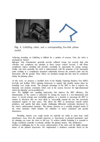
ground in order to make forward progress. To address this, we define a virtual obstacle
function, _( x), which is safely below the terrain around candidate foothold regions, and
above the ground in regions where we do not allow foot contact (illustrated in Figure 6). In
our previous experience with planning walking gaits (Byl et al. 2008; Byl and Tedrake 2009),
it was clear that challenging rough terrain could be separated into regions with useful
candidate footholds, as opposed to regions where footholds would be more likely to cause a
failure. Therefore, we had developed algorithms to pre-process the terrain to identify these
candidate foothold regions based on some simple heuristics, and we could potentially use the
same algorithms here to construct _( x). However, in the current work, which makes heavy
use of the motion primitive described in the following sections, we found it helpful to
construct separate virtual obstacles, _m( x), parameterized by the motion primitive, m, being
performed. Once the virtual obstacles became motion primitive dependent, we had success
with simple virtual obstacles as illustrated in Figure 6. The collision function illustrated is
defined relative to the current position of the feet. In the case shown in the figure, the virtual
function forces the swing leg to lift up and over the terrain, and ensures that the back foot
does not slip, which characterizes a successful portion of a bound. As soon as the front feet
touch back down to the ground after completing this part of the bound, a new collision
function is defined, which takes into account the new footholds, and forces the back feet to
make forward progress in the air.
We are now ready to formulate the motion planning problem for LittleDog bounding: find a
feasible solution, {x[0], u[0], x[1], u[1], . . . , x[N]}, which starts in the required initial
conditions, satisfies the dynamics of the
model, x[n + 1] = f( x[n], u[n]), avoids collisions with the virtual obstacles, _( x), does not
violate the bounds on joint positions, velocities, accelerations, and torques, and reaches the
goal position.
Given this problem formulation, it is natural to consider a sample-based motion planning
algorithms such as RRTs due to their success in high-dimensional robotic planning problems
involving complex geometric constraints (LaValle and Branicky 2002). However, these
algorithms perform poorly when planning in state space (where the dynamics impose
“differential constraints”) (Cheng 2005; LaValle 2006), especially in high dimensions.When
applied directly to building a forward tree for this problem, they take prohibitive amounts of
time and fail to make any substantial progress towards the goal. In the following sections, we
describe three modifications to the basic algorithm. First, we describe a parameterized “half-
bound” motion primitive which reduces the dimensionality of the problem. Second, we
describe the Reachability-Guided RRT, which dynamically changes the sampling distribution

13. and distance metric to address differential constraints and discontinuous motion primitive
dynamics. Finally, we describe a mechanism for sampling with a Voronoi bias in the lower-
dimensional task space defined by the motion primitive. All three of these approaches were
necessary to achieve reasonable run-time performance of the algorithm.
4.2. Macro Actions/Motion Primitive
The choice of action space, e.g. how an action is defined for the RRT implementation, will
affect both the RRT search efficiency, as well as completeness guarantees, and, perhaps most
importantly, path quality. In the case of planning motions for a five-link planar arm with four
actuators, a typical approach may be to consider applying a constant torque (or some other
simple action in joint space) that is applied for a short constant time duration, _T. One
drawback of this method is that the resulting trajectory found by the RRT is likely be jerky. A
smoothing/optimization postprocessing step may be performed, but this may require
significant processing time, and there is no guarantee that the local minima near the original
trajectory is sufficiently smooth. Another drawback of using a constant time step with such
an action space is that in order to ensure completeness,
_T should be relatively small (for LittleDog bounding, 0.1 seconds seems to be appropriate).
Empirically,
however, the search time increases approximately as 1/_T, so this is a painful trade-off. For a
stiff PD-controlled robot, such as LittleDog, itmakes sense to have the action space
correspond directly to position commands. To do this, we generate a joint trajectory by using
a smooth function, G, that is parameterized by the initial joint positions and velocities, [q( 0) ,
˙q( 0)], a time for the motion, _Tm, and the desired end joint positions and velocities,
[qd(_Tm) , ˙qd(_Tm)]. This action set requires specifying two numbers for each actuated
degree of freedom: one for the desired end position and one for the desired end velocity. A
smooth function generator which obeys the end point constraints, for example a cubic-spline
interpolation, produces a trajectory which can be sampled and sent to the PD controller.

14. 4.3. Reachability-guided RRT Overview
Sample-based planning methods such as the RRT can bevery fast for certain applications.
However, such algorithms depend on a distance metric to determine distance from samples to
nodes in the tree. The Euclidean distance metric is easy to implement, and works well for
holonomic path planning problems, but it breaks down when constraints imposed by the
governing equations of motion restrict the direction that nodes can grow in. To deal with this,
we developed a modified version of the RRT algorithm called the Reachability-Guided RRT
(RG-RRT) (Shkolnik et al. 2009). The algorithm uses rejection sampling, which was
previously shown to be beneficial for growing trees in configuration space through narrow
tunnels (Yershova et al. 2005). Reachability guidance extends this idea to planning for
dynamic systems in state space. The RG-RRT biases the RRT search toward parts of state
space that are locally reachable from the tree. Reachability information is stored in each node
in the tree; the algorithm works by sampling and then measuring the Euclidean (or scaled-
Euclidean) distance to each node in the tree, as well as to each reachable set of the tree. If a
sample is closer to the tree itself, rather than to the reachable set of the tree, then there are no
actions which are able to extend that node in the direction of the sample. This sample–node
pair is therefore not useful for exploration, and is discarded. On the other hand, if the sample
is closer to a reachable region, the parent node in the tree, which generated the closest
reachable region, is grown towards the sample. Thus, by keeping track of locally reachable
parts of the tree and using a simple Euclidean-type distance metric, the algorithm is able to
overcome many of the inherent difficulties when implementing an RRT for dynamic systems.
In this work, we show that the RG-RRT algorithm can be useful for motion planning in a
system with motion

15. primitives. Conceptually, a motion primitive in a dynamic system is one which occurs over a
fairly substantial duration of time, e.g. an action which moves the system from one state to
another state that is relatively distant from the current state. Therefore, the states produced by
taking macro actions or motion primitives may be discontinuous or even discrete in relation
to a generating state, which would invalidate the use of a proper Euclidean distance metric
that assumes a smooth continuous space of actions. The idea of Reachability can be an
especially powerful notion for sample-based planning in the context of macro actions, as the
reachable region does not have to be local to its parent node. A continuous motion primitive
action space can be approximated by sampling in the action space, resulting in a discrete set
of reachable nodes, which might be far in state space from their parent node. This idea
suggests that the RG-RRT also naturally extends to models with hybrid dynamics, simply by
sampling actions and integrating through the dynamics when generating the
reachable set.
4.4. Approximating the Reachable Set
We have shown that Reachability Guidance can improve RRT planning time in underactuated
systems such as the torque-limited pendulum and Acrobot (Shkolnik et al. 2009). In those
systems, the reachable set was approximated by discretizing the action space. However, to
achieve LittleDog bounding, even a reduced four-dimensional action space becomes too large
to discretize efficiently. For example, using only three actions per dimension (and assuming a
constant motion primitive time step), there would be 81 actions to apply and simulate in order
to approximate the reachable set for each node. Instead of discretizing in such a high
dimensional action space, the reachable set can be approximated by understanding the failure
modes of bounding. Failures may occur primarily in one of three ways: (1) the robot has too
much energy and falls over; (2) the robot has too little energy, so the stance foot never leaves
the ground, violating our assumption that one foot always leaves the ground in a bounding
gait; or (3) a terrain collision occurs. In the case when the system has a lot of kinetic energy,
the best thing to do is to straighten all of the limbs, which raises the COM and converts the
kinetic energy into potential energy. At the other extreme, if the robot does not have much
kinetic energy, an action that lowers the COM while accelerating the limbs inwards tends to
produce a rotational moment, if it is possible to do so. Thus, two extreme motions can be
generated, for each phase of bounding, which prevent the two common failure modes. The
reachable set is then generated by interpolating joint positions between the two extremes.
This one-dimensional discretization is usually rich enough to capture the energy related
failure modes and generate bounds which strike the right balance to continue bounding
further.
The reachable set helps the RG-RRT to plan around Regions of Inevitable Collisions (RIC)
(LaValle and Kuffner 2001; Fraichard and Asama 2003; Fraichard 2007; Chan et al. 2008).
Nodes which have empty reachable sets, which may occur because the node has too much or
too little energy, in the case of LittleDog bounding, are in XRIC, even if the node itself is
collision free (Xfree). The RG-RRT takes advantage of this, because when a node has an
empty reachable set, the node serves as a “blocking” function for sampling. Owing to the
rejection sampling of the RG-RRT, such a node cannot be expanded upon, and any samples
that map to this node will be discarded, encouraging sampling in other areas that can be
expanded.

16. 4.5. Sampling in Task Space
In the RRT algorithm, sampling is typically performed uniformly over the configuration
space. An action is chosen which is expected to make progress towards the sample. The
sampling creates a Voronoi bias for fast exploration by frequently selecting nodes of the tree
near unexplored regions, while occasionally refining within explored regions. We have
previously shown that the Voronoi bias can be implemented in the configuration (or state)
space or alternatively the bias can be in a lower-dimensional task space (Shkolnik and
Tedrake 2009). This can be achieved simply by sampling in task space, and finding the node
in the configuration-space tree, the projection of which is closest to the task-space sample.
Reducing the dimensionality of the search with a task space Voronoi bias can significantly
improve search efficiency and, if done carefully, does not have an impact on the
completeness of the algorithm.
4.6. Simulation Results
In this section, we have presented three modifications tothe standard implementation of the
RRT to plan bounding motions with LittleDog: (1) a simple motion primitive; (2) reachability
guidance; and (3) task-space biasing. Each of these components could be implemented
separately, but they worked particularly well when combined. To show this, we qualitatively
compare results by applying various combinations of these modifications.
4.7. Experimental Results
In experiments with the real robot, open-loop execution of the motion plan found by the RRT
quickly diverged with time from the model predictions, even on flat terrain. Trajectories are
unstable in the sense that given the same initial conditions on the robot and a tape of position
commands to execute, the robot trajectories often diverge, sometimes catastrophically. To
demonstrate the feasibility of using the motion primitives described in this paper, these
motion primitives were used to achieve a short bound sequence over the log terrain. Unlike in
the model, the actual logs are not planar. To address this, tracks were laid on the logs
corresponding to the stance width of the robot along the terrain. The planner was constrained
to only allow foot holds where the points on adjacent tracks were of the same height. With
some tuning, the motion primitives produced bounding over the logs on the real robot, shown
in Figure 14. This trajectory was successful approximately 20% of the time, even though care
was taken to have the same initial position for each trial.
5. Feedback Stabilization.
Figure 15 shows the sensing and control environment for LittleDog. For most feedback
control methods, one selects a state space suitable for the task at hand, and uses an observer
to construct an estimate of the current state using available measurements. An accurate
observer requires a good dynamical model of the robot and knowledge of the characteristics
(e.g. delays and noise) of each measurement. Having estimated the state, the controller must
select an action to take, which stabilizes the bounding motion. This is a non-trivial task
because of the highly non-linear nature of the dynamics and the limited control authority
available for the unactuated coordinate. Several recent efforts in control of underactuated

17. systems have found success in taking a three-stage approach (Westervelt et al. 2003; Song
and Zefran 2006; Westervelt et al. 2007; Shiriaev et al. 2008; Manchester et al. 2009):.
5.1. Selection of Projection and Optimization Weights
Using the transverse-LQR controller we were able to achieve stable bounding in simulations
with several types of perturbations. The success of the method is heavily dependent on a
careful choice of both the projection P( x) and the weighting matrices Q and R.
For the projection, LittleDog was represented as a floating five-link chain but in a new
coordinate system: the first coordinate was derived by considering the vector from thepoint of
contact of the stance foot and the COM of the robot. The angle θ of this line with respect to
the horizontal was the first generalized coordinate. The remaining coordinates were the
angles of the four actuated joints, and the ( x, y) position of the non-stance (swing) foot. In
this coordinate system, the projection on to the target trajectory was taken to be the closest
point under a weighted Euclidean distance, with heaviest weighting on θ, somewhat lighter
weighting on ˙ θ, and much lighter weighting on the remaining coordinates.
5.2. Simulation Results
We have simulated the transverse-linearization controller with a number of RRT-generated
bounding trajectories. For some trajectories over flat terrain in simulation, we were able to
stabilize these trajectories even when adding a combination of: (1) slight Gaussian noise to
the state estimate (σ = 0.01 for angles, σ = 0.08 for velocities), (2) significant velocity
perturbations up to 1 rad s−1 after each ground impact, (3) model parameter estimation error
of up to 1 cm in the main body COM position, and (4) delays of up to 0.04 seconds. In this
section we will show some results of stabilization on two example terrains: bounding up
stairs and bounding over logs.
5.3. Experimental Results
We are currently working to implement the transverse-LQR system on the real robot. At
present, the main difficulty stems from the measurement system on the experimental
platform, seen in Figure 15. In order to implement our controller, we must have knowledge of
the state of the robot, and in experiments this is derived from a combination of an on-board
IMU, motor encoders, and the motion-capture
system.
6. Concluding Remarks and Future Directions
In this paper, we have demonstrated motion planning forthe LittleDog quadruped robot to
achieve bounding on very rough terrain. The robot was modeled as a planar system with a 16-
dimensional state space. A physics-based simulation was developed and identified using data
from the real robot. An efficient RRT-based planner was implemented. This planner used
motion primitives to reduce the size of the action space, and also to produce smooth
trajectories without an optimization step. Task-space guidance was implemented by sampling
from a five-dimensional subset of the state space. The reduction in sampling dimension

18. ignores pitch, vertical position, and velocities which significantly improves search efficiency.
To handle challenging dynamic constraints associated with bounding, we used reachability
guidance, so that random samples were chosen such that they were closer to reachable
regions of the tree, rather than to the tree itself. Doing so increases the likelihood that the
expansion step of the RRT algorithm can make progress in the direction of the sample, which
dramatically improves RRT performance. The RRT motion planner was demonstrated to
achieve bounding over steps and over logs, with terrain height differences corresponding to
approximately 50% of the leg length. Without reachability guidance, 12 hours was not
sufficient to plan in the otherwise identical conditions. Using task-space biasing and
reachability guidance, we were able to plan within minutes. A primary reason for this is that a
standard RRT implementation does not look ahead. Many of the nodes on the outer edges of
the tree (the exact nodes which the Voronoi bias selects most often, because they are near the
unexplored regions
of state space) correspond to nodes that are either incapable of bounding on the next step
because not enough energy is carried over, or have too much energy and no possible action
could be applied on the next step to keep the robot from falling over. Expanding on these
nodes is futile, but the standard RRT will try to expand them repeatedly causing the algorithm
to fail to find a plan.
7 Acknowledgements
This work was supported by the DARPA Learning Locomotion program (AFRL contract #
FA8650-05-C-7262). The authors would also like to thank Sara Itani for her help during
Phase III, especially in tuning an open-loop bounding gate.
8 References
Altendorfer R, Moore N, Komsuoglu H, Buehler M, Brown HB, McMordie D, et al. (2001)
RHex: A biologically inspired
hexapod runner. Autonomous Robots 11: 207–213.
Berges P and Bowling A (2006) Rebound, slip, and compliance in the modeling and analysis
of discrete impacts in legged
locomotion. Journal of Vibration and Control 12: 1407–1430.
Byl K, Shkolnik A, Prentice S, Roy N and Tedrake R (2008) Reliable dynamic motions for a
stiff quadruped. In Proceedings of the 11th International Symposium on Experimental
Robotics (ISER), Athens, Greece.
Byl K and Tedrake R (2009) Dynamically diverse legged locomotion for rough terrain. In
Proceedings of the IEEE/RAS International Conference on Robotics and Automation (ICRA
09), Kobe, Japan.
Chan N, Kuffner J and Zucker M (2008) Improved motion planning speed and safety using
regions of inevitable collision. In
17th CISM-IFToMM Symposium on Robot Design, Dynamics, and Control (RoManSy’08),
Tokyo, Japan.

19. Cheng P (2005) Sampling-based Motion Planning with Differential Constraints. Ph.D. thesis,
University of Illinois at Urbana- Champaign, IL.
Chestnutt J, Lau M, Cheung KM, Kuffner J, Hodgins JK and Kanade T (2005) Footstep
planning for the honda asimo humanoid. In Proceedings of the IEEE/RAS International
Conference on Robotics and Automation (ICRA 05), Barcelona.