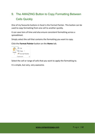
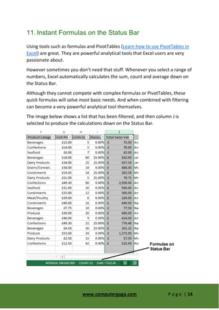
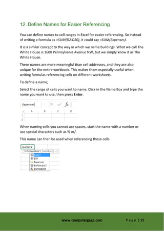
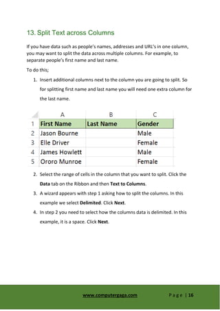
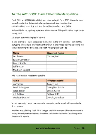
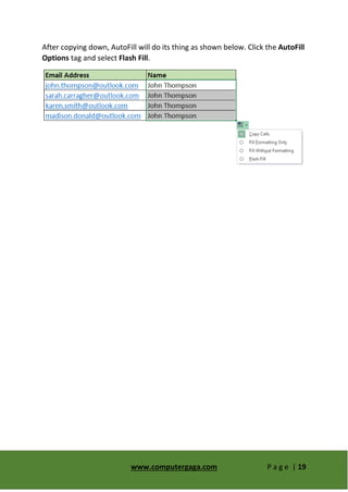
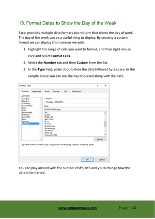
Excel Excellence (Microsoft Excel training that "sticks"): FormulasLaura Winger
Microsoft Excel is one of the most powerful tools, and if you use Excel on a regular basis for your job, chances are you are under utilizing it and could increase your productivity and free up hours each week with improved Excel skills. My Excel Excellence courses provide hands-on experience with realistic business examples and simplified explanations. Become a whiz at VLookUp's, PivotTables, and even program your own Macros! This slide deck is a preview from my first session on Formulas. Formulas are used for more than math, they can be used for re-formatting data, extracting data and putting data together (“concatenating”). Learn how to harness the power of Excel and put the computer to work for you!
SEE MORE, INCLUDING A FREE TRIAL, AT: www.PivotTable-Pro.com
This video introduces you to Microsoft Excel 2013 and its program window.
Free Excel Training Course: http://www.SpreadsheetTrainer.com
Contents:
***Introduction - What is Microsoft Excel?***
***The Excel Program Window***
Program Window - Border & Title
How to Maximise the Excel Window
How to Minimise the Excel Window
How to Close the Excel Window
***The Excel Ribbon***
How to Hide & Show the Ribbon
What is the Excel Ribbon?
What are Groups?
What are Command Buttons?
What are Smart Tags?
What are Dialog Boxes?
What is the File tab & Backstage Menu?
The Excel Ribbon Shrinks When you Resize the Window
***Other Program Window Elements***
What is the Quick Access Toolbar?
What is the Name Box?
What is the Formula Bar?
How to Resize the Formula Bar
What is the Status bar?
Where are the View shortcuts?
How to use the Scroll Bars
What is the Spreadsheet Area?
What is the Mini Toolbar?
SEE MORE, INCLUDING A FREE TRIAL, AT: www.PivotTable-Pro.com
This video teaches basic data entry and editing in Excel.
Free Excel Training Course: http://www.SpreadsheetTrainer.com
Contents:
***Data Entry in Excel***
How to Enter Data into a Cell
The Enter Status Mode
How to Structure Data
How to Exit a Cell with the Keyboard and Formula Bar
How to Cancel Cell Changes
How to Use Undo/Redo
How to Use AutoComplete
How to insert a New Line in a Cell
How to Enter a Block of Data using a Range
How to Instantly Insert Values into a Range
***Formulas vs Values vs Text***
The Differences between formulas, values and text
Entering negative numbers with minus sign or ()
Entering Dates & Times
Entering Percentages & Currencies
How Excel treats Text Entries vs Value Entries.
***Editing or Deleting Existing Entries***
How to Overwrite an Existing Entry
How to Edit an Existing Entry
The Edit Status Mode
How to delete a Current Entry with Delete & Clear Contents
SEE MORE, INCLUDING A FREE TRIAL, AT: www.PivotTable-Pro.com
This video shows basic worksheet elements and navigation in Excel.
Free Excel Training Course: http://www.SpreadsheetTrainer.com
Contents:
***The Excel Worksheet ***
What is a cell?
What is a row?
What is a column?
***Selecting & Navigating***
What is the selected cell?
How to select a cell in the Excel worksheet
How to use the GoTo function
How to navigate with page up & page down,
How to navigate with Alt+page up & Alt+page down,
Navigating with Ctrl+arrow, Home, & Ctrl+Home
***Ranges***
What is a range?
How to select a range with the mouse and keyboard
How to select a range with Ctrl+Shift+Arrow
What is the active cell?
How to select nonadjacent cells.
Referring to range addresses.
The site present the assignment to the students in well- structured manner including all the information in the simplest form, so that students need not spend extra time and effort in completion of the assignment and along with these they can also gain all the content engraved in the brain.
SEE THE FULL, FREE EXCEL 2013 TRAINING COURSE AT WWW.PIVOTEXCEL.COM
This presentation introduces you to basic Excel function syntax and usage, and runs through some basic mathematical functions.
Contents:
***Standard Function Syntax***
Elements of an Excel Function
Inputting Function Arguments
AutoComplete for Functions
***Basic Numerical Functions***
Using Sum(), Max(), Min(), Average() and Count()
Functions Update Automatically as Arguments Change.
Using Comma and Colon to Reference Cells & Ranges.
Using Cell References, Values, Formulas or other Functions as Arguments.
Inserting a Formula into Many Cells at Once with CTRL+ Enter.
***The AutoSum & Quick Analysis Feature***
The Autosum Tool
The Quick Analysis Feature
***Function Library & Insert Function Tool***
Using the ‘Insert Function’ Tool.
***Editing & Deleting Functions***
Editing & Deleting Functions with Mouse & Keyboard
Editing a Function with the Insert Function Tool
MS Excel Learning for PPC Google AdWords Training CourseRanjan Jena
MS Excel learning to get expertise in Google AdWords training course. Learn all important tips and techniques in MS Excel for your fast and easy approach to Google AdWords analysis and reporting formats.
Ranjan Jena conducts Adwords Training session in Bangalore, currently with more than 45 students already graduated under his guidance and mentorship. For any training need, you can directly reach him at +91-7760969452
These are MS Excel Tips and tricks you might not know, which will advance your skills in using Excel, also these tips and tricks are the main Job exams questions
to perform 3 tasks that will generate 3 data sets, which are as follows: (a) Dataset 1: Student data; (b) Dataset 2: Car data; and (c) Dataset 3: Employee's details. Explore and simulate the built-in functions of a spreadsheet app for data cleaning.
NCompass Live - Aug. 22, 2018
http://nlc.nebraska.gov/ncompasslive/
Microsoft Excel has a variety of uses in the library world from keeping track of budgets or managing program registrations to viewing circulation or collection statistics. Learn some hints and tips for working with already existing spreadsheets as well as building your own. We’ll also take a look at Google Sheets and see how that compares with Excel.
Presenter: Megan Boggs, Seward (NE) Memorial Library.
OpenFOAM solver for Helmholtz equation, helmholtzFoam / helmholtzBubbleFoamtakuyayamamoto1800
In this slide, we show the simulation example and the way to compile this solver.
In this solver, the Helmholtz equation can be solved by helmholtzFoam. Also, the Helmholtz equation with uniformly dispersed bubbles can be simulated by helmholtzBubbleFoam.
How Does XfilesPro Ensure Security While Sharing Documents in Salesforce?XfilesPro
Worried about document security while sharing them in Salesforce? Fret no more! Here are the top-notch security standards XfilesPro upholds to ensure strong security for your Salesforce documents while sharing with internal or external people.
To learn more, read the blog: https://www.xfilespro.com/how-does-xfilespro-make-document-sharing-secure-and-seamless-in-salesforce/
Designing for Privacy in Amazon Web ServicesKrzysztofKkol1
Data privacy is one of the most critical issues that businesses face. This presentation shares insights on the principles and best practices for ensuring the resilience and security of your workload.
Drawing on a real-life project from the HR industry, the various challenges will be demonstrated: data protection, self-healing, business continuity, security, and transparency of data processing. This systematized approach allowed to create a secure AWS cloud infrastructure that not only met strict compliance rules but also exceeded the client's expectations.
top nidhi software solution freedownloadvrstrong314
This presentation emphasizes the importance of data security and legal compliance for Nidhi companies in India. It highlights how online Nidhi software solutions, like Vector Nidhi Software, offer advanced features tailored to these needs. Key aspects include encryption, access controls, and audit trails to ensure data security. The software complies with regulatory guidelines from the MCA and RBI and adheres to Nidhi Rules, 2014. With customizable, user-friendly interfaces and real-time features, these Nidhi software solutions enhance efficiency, support growth, and provide exceptional member services. The presentation concludes with contact information for further inquiries.
Why React Native as a Strategic Advantage for Startup Innovation.pdfayushiqss
Do you know that React Native is being increasingly adopted by startups as well as big companies in the mobile app development industry? Big names like Facebook, Instagram, and Pinterest have already integrated this robust open-source framework.
In fact, according to a report by Statista, the number of React Native developers has been steadily increasing over the years, reaching an estimated 1.9 million by the end of 2024. This means that the demand for this framework in the job market has been growing making it a valuable skill.
But what makes React Native so popular for mobile application development? It offers excellent cross-platform capabilities among other benefits. This way, with React Native, developers can write code once and run it on both iOS and Android devices thus saving time and resources leading to shorter development cycles hence faster time-to-market for your app.
Let’s take the example of a startup, which wanted to release their app on both iOS and Android at once. Through the use of React Native they managed to create an app and bring it into the market within a very short period. This helped them gain an advantage over their competitors because they had access to a large user base who were able to generate revenue quickly for them.
Advanced Flow Concepts Every Developer Should KnowPeter Caitens
Tim Combridge from Sensible Giraffe and Salesforce Ben presents some important tips that all developers should know when dealing with Flows in Salesforce.
Accelerate Enterprise Software Engineering with PlatformlessWSO2
Key takeaways:
Challenges of building platforms and the benefits of platformless.
Key principles of platformless, including API-first, cloud-native middleware, platform engineering, and developer experience.
How Choreo enables the platformless experience.
How key concepts like application architecture, domain-driven design, zero trust, and cell-based architecture are inherently a part of Choreo.
Demo of an end-to-end app built and deployed on Choreo.
Strategies for Successful Data Migration Tools.pptxvarshanayak241
Data migration is a complex but essential task for organizations aiming to modernize their IT infrastructure and leverage new technologies. By understanding common challenges and implementing these strategies, businesses can achieve a successful migration with minimal disruption. Data Migration Tool like Ask On Data play a pivotal role in this journey, offering features that streamline the process, ensure data integrity, and maintain security. With the right approach and tools, organizations can turn the challenge of data migration into an opportunity for growth and innovation.
Quarkus Hidden and Forbidden ExtensionsMax Andersen
Quarkus has a vast extension ecosystem and is known for its subsonic and subatomic feature set. Some of these features are not as well known, and some extensions are less talked about, but that does not make them less interesting - quite the opposite.
Come join this talk to see some tips and tricks for using Quarkus and some of the lesser known features, extensions and development techniques.
Software Engineering, Software Consulting, Tech Lead.
Spring Boot, Spring Cloud, Spring Core, Spring JDBC, Spring Security,
Spring Transaction, Spring MVC,
Log4j, REST/SOAP WEB-SERVICES.
Globus Connect Server Deep Dive - GlobusWorld 2024Globus
We explore the Globus Connect Server (GCS) architecture and experiment with advanced configuration options and use cases. This content is targeted at system administrators who are familiar with GCS and currently operate—or are planning to operate—broader deployments at their institution.
Large Language Models and the End of ProgrammingMatt Welsh
Talk by Matt Welsh at Craft Conference 2024 on the impact that Large Language Models will have on the future of software development. In this talk, I discuss the ways in which LLMs will impact the software industry, from replacing human software developers with AI, to replacing conventional software with models that perform reasoning, computation, and problem-solving.
A Comprehensive Look at Generative AI in Retail App Testing.pdfkalichargn70th171
Traditional software testing methods are being challenged in retail, where customer expectations and technological advancements continually shape the landscape. Enter generative AI—a transformative subset of artificial intelligence technologies poised to revolutionize software testing.
Cyaniclab : Software Development Agency Portfolio.pdfCyanic lab
CyanicLab, an offshore custom software development company based in Sweden,India, Finland, is your go-to partner for startup development and innovative web design solutions. Our expert team specializes in crafting cutting-edge software tailored to meet the unique needs of startups and established enterprises alike. From conceptualization to execution, we offer comprehensive services including web and mobile app development, UI/UX design, and ongoing software maintenance. Ready to elevate your business? Contact CyanicLab today and let us propel your vision to success with our top-notch IT solutions.
Enhancing Research Orchestration Capabilities at ORNL.pdfGlobus
Cross-facility research orchestration comes with ever-changing constraints regarding the availability and suitability of various compute and data resources. In short, a flexible data and processing fabric is needed to enable the dynamic redirection of data and compute tasks throughout the lifecycle of an experiment. In this talk, we illustrate how we easily leveraged Globus services to instrument the ACE research testbed at the Oak Ridge Leadership Computing Facility with flexible data and task orchestration capabilities.
Developing Distributed High-performance Computing Capabilities of an Open Sci...Globus
COVID-19 had an unprecedented impact on scientific collaboration. The pandemic and its broad response from the scientific community has forged new relationships among public health practitioners, mathematical modelers, and scientific computing specialists, while revealing critical gaps in exploiting advanced computing systems to support urgent decision making. Informed by our team’s work in applying high-performance computing in support of public health decision makers during the COVID-19 pandemic, we present how Globus technologies are enabling the development of an open science platform for robust epidemic analysis, with the goal of collaborative, secure, distributed, on-demand, and fast time-to-solution analyses to support public health.
Into the Box Keynote Day 2: Unveiling amazing updates and announcements for modern CFML developers! Get ready for exciting releases and updates on Ortus tools and products. Stay tuned for cutting-edge innovations designed to boost your productivity.
2. www.computergaga.com P a g e | 2
About Me
Hello everyone,
My name is Alan Murray. I live in
Ipswich in the United Kingdom with my
wife and 2 children.
I work as an IT Trainer and have done
for the last 20 years.
Working as an IT Trainer, I visit many
organisations to train their staff in the
use of Excel.
This means I get to meet many
wonderful people and also get a good understanding of what Excel skills
users’ need, and want to know.
I set up Computergaga to help spread these in-demand tips and skills to
others.
I’m an Excel enthusiast and am always learning myself so encourage
comments and community spirit on my blog. I hope to see you there.
3. www.computergaga.com P a g e | 3
Want to be an Excel Superhero?
Learn all the skills you need to know to be an Excel Expert
IF Functions
PivotTables
VLOOKUP
Charts
Conditional Formatting
Manipulating Text
Macros
And much, much more
4. www.computergaga.com P a g e | 4
1. Adding Numbers with Leading Zeros
When entering numbers into a cell in Excel, you may wish to keep the leading
zeros. Examples might include when entering phone numbers, or employee
ID’s.
However Excel will not allow this and will remove any leading zeros. For
example, if you typed 002 into Excel, it would display 2. The zeros are deemed
redundant.
There are two methods we can use to make Excel keep the leading zeros. One
way is to enter them as text, and the other is to format them with zeros (this
approach will keep the value numeric).
To enter a number as text (such as a phone number), we can simply precede
the number with a single quotation ‘. This tells Excel that you have typed a
number, but want it stored as text. Excel will react like in the image below.
You can see in the Formula Bar that a single quotation was typed. In the cell a
warning icon is displayed, and when I click on it I am provided with a quick way
to convert it to a number if this was a mistake.
To remove the warning and keep it as text with the leading zero, click Ignore
Error.
Another way to enter a number with leading zeros is to customise the
formatting of the number. Let’s imagine that we are entering employee ID’s
which are exactly 8 characters in length.
1. Select the range of cells you want to apply the formatting to.
5. www.computergaga.com P a g e | 5
2. Right mouse click on the selected cells and click Format Cells, or press
Ctrl + 1 (neat Excel shortcut there ).
3. Select the Number tab, Custom from the list on the left and enter
00000000 (eight zeros) into the Type box.
In the sample area of the image above you can see Excel placing a 0 at the start
of the employee ID, which would otherwise only be 7 numbers in length.
The 0’s enter into the Type box force Excel to display a number. Therefore if
we do not enter one, Excel puts in a 0.
6. www.computergaga.com P a g e | 6
2. Restrict Values with Data Validation
When manipulating, analysing and reporting on data, these tasks will only be
as successful as the data itself. There is no point being a PivotTable guru if your
colleagues are mistyping names, and not entering dates correctly.
The Data Validation tool in Excel is great for ensuring the data being entered is
clean and correct. You can write all kinds of validation rules to check data,
however the most common use of Data Validation is to create a drop down list
of options.
Let’s look at how to do this;
1. Select the range of cells you want to apply the Data Validation rules to.
2. Click the Data tab and then Data Validation.
3. On the Settings tab, select List from the Allow options.
4. You can now enter the list entries into the Source box separating each
one with a comma (shown in image below).
Or
Select a range of cells that contains the entries for the list.
7. www.computergaga.com P a g e | 7
And we now have a list in each of the cells that you selected (Check out how to
create multiple dependent drop down lists).
You can type in the cells, but if you try and enter anything that is not in the list,
Excel will refuse it.
3. Navigate Large Lists Using the Keyboard
When working with large lists even the simple art of navigation can be
awkward and cumbersome, unless you know some trusty shortcuts.
Pressing Ctrl + Arrow key will jump you to the end of that row or column
(it stops at the first empty cell, so depends how your list is structured).
Ctrl + Home or End will jump you to the first cell of the table (Home), or
the last cell of the table (End).
By also pressing the Shift key during these shortcuts, it will select the
cells.
Pressing Ctrl + Shift + 8 selects the current region. This means it selects
all the cells from the current range you are in.
8. www.computergaga.com P a g e | 8
4. Quickly Enter Todays Date
Do you have to enter todays date often?
Then you will love this keyboard shortcut that enters it for you.
It is Ctrl + ;
Enjoy!
That will save time and also ensure there are no mistakes entering it.
5. Insert Multiple Rows or Columns at Once
Excel will insert the same number of rows and columns that you have selected.
So if you want to insert four new rows after row 8;
Select rows 9 to 12.
Right mouse click on the selected rows and click Insert.
The same technique works for columns.
9. www.computergaga.com P a g e | 9
6. Select All the Formulas on a Sheet
Excel has a wonderful feature called Go To Special which enables you to select
cells on a spreadsheet that meet certain conditions.
Possibly it’s most common use is to select ALL the formulas on the sheet.
You may be doing this so that you can protect the cells with formulas, or
change the background colour of them.
Click the Home tab, then Find & Select and then Formulas.
Click the Go To Special option from Find & Select to see all of the options that
this amazing tool has. Other GREAT options include selecting all the blank cells
in a range, those with Data Validation rules or those containing formula error.
10. www.computergaga.com P a g e | 10
7. Copy Formulas to the Bottom of a List WITHOUT
Dragging
When working with large lists, dragging the Fill handle to copy formulas can be
awkward and frustrating.
Great News.
Double click the Fill handle and Excel will copy it to the bottom of the list for
you. AMAZING!
Excel will use the column to the left as a guide. When that column ends (at a
blank cell), your copying will stop.
11. www.computergaga.com P a g e | 11
8. Switch a List from Rows to Columns
In an ideal world for Excel, your data should be in a classic table format. By this
I mean that your headers will be in the top row and each row will be a record,
with the columns as type of information about that record.
However especially when importing data from databases and online services it
does not always appear that way.
Fortunately Excel provides a simple way to switch your data from rows to
columns and it’s called Transpose.
1. Select the range of cells you want to rotate.
2. Click Home and then Copy or press Ctrl + C.
3. Click in a destination cell (you can always move it afterwards).
4. Click the Home tab, the list arrow of the Paste button and select the
Transpose option.
12. www.computergaga.com P a g e | 12
9. The AMAZING Button to Copy Formatting Between
Cells Quickly
One of my favourite buttons in Excel is the Format Painter. This button can be
used to copy formatting from one cell to another quickly.
It can save tons of time and also ensure consistent formatting across a
spreadsheet.
Simply select the cell that contains the formatting you want to copy.
Click the Format Painter button on the Home tab.
Select the cell or range of cells that you want to apply the formatting to.
It is simple, but very, very awesome.
13. www.computergaga.com P a g e | 13
10. Removing the Formula from a Cell by Pasting
Values Only
When copying and pasting cells, Excel pastes everything about the cell
including its formula, formatting and validation rules.
Fortunately there is a feature called Paste Special which enables us to choose
which elements of the copied data that we want to paste.
Two of the most common Paste Special options are paste Values and paste
Values and Number Formatting.
These options are great when you do not want a formula to calculate anymore.
You can copy and paste Values to effectively keep the result, but remove the
underlying formula.
These pasting options also come in handy when sending spreadsheets to
clients and other external recipients for whom you do not wish to view your
formulas.
14. www.computergaga.com P a g e | 14
11. Instant Formulas on the Status Bar
Using tools such as formulas and PivotTables (Learn how to use PivotTables in
Excel) are great. They are powerful analytical tools that Excel users are very
passionate about.
However sometimes you don’t need that stuff. Whenever you select a range of
numbers, Excel automatically calculates the sum, count and average down on
the Status Bar.
Although they cannot compete with complex formulas or PivotTables, these
quick formulas will solve most basic needs. And when combined with filtering
can become a very powerful analytical tool themselves.
The image below shows a list that has been filtered, and then column J is
selected to produce the calculations down on the Status Bar.
15. www.computergaga.com P a g e | 15
12. Define Names for Easier Referencing
You can define names to cell ranges in Excel for easier referencing. So instead
of writing a formula as =SUM(D2:D20), it could say =SUM(Expenses).
It is a similar concept to the way in which we name buildings. What we call The
White House is 1600 Pennsylvania Avenue NW, but we simply know it as The
White House.
These names are more meaningful than cell addresses, and they are also
unique for the entire workbook. This makes them especially useful when
writing formulas referencing cells on different worksheets.
To define a name;
Select the range of cells you want to name. Click in the Name Box and type the
name you want to use, then press Enter.
When naming cells you cannot use spaces, start the name with a number or
use special characters such as % or/.
This name can then be used when referencing those cells.
16. www.computergaga.com P a g e | 16
13. Split Text across Columns
If you have data such as people’s names, addresses and URL’s in one column,
you may want to split the data across multiple columns. For example, to
separate people’s first name and last name.
To do this;
1. Insert additional columns next to the column you are going to split. So
for splitting first name and last name you will need one extra column for
the last name.
2. Select the range of cells in the column that you want to split. Click the
Data tab on the Ribbon and then Text to Columns.
3. A wizard appears with step 1 asking how to split the columns. In this
example we select Delimited. Click Next.
4. In step 2 you need to select how the columns data is delimited. In this
example, it is a space. Click Next.
17. www.computergaga.com P a g e | 17
5. In the 3rd
and final step you can change the format of the columns. In
this example it is not necessary as each column is a General format. Click
Finish.
The Text to Columns feature is useful for the most common situations at
splitting data from a column. Check out this tutorial for 3 more advanced
techniques at separating text in a column.
18. www.computergaga.com P a g e | 18
14. The AWESOME Flash Fill for Data Manipulation
Flash Fill is an AMAZING tool that was released with Excel 2013. It can be used
to perform typical data manipulation tasks such as extracting text,
concatenating, reversing text and formatting numbers and dates.
It does this by recognising a pattern when you are filling cells. It is a huge time-
saving tool.
Let’s look at two examples of its use.
In this example, I want to reverse the names in the first column. I can do this
by typing an example of what I want (shown in the image below), selecting the
cell and clicking the Data tab and Flash Fill (or press Ctrl + E).
And Flash Fill will repeat the pattern.
In this example, I want to extract the names from the email addresses in the
first column.
Another way of using Flash Fill is to type the first example of what you want it
to do, then copy that down to the other cells in the list in the usual way with
the AutoFill handle.
19. www.computergaga.com P a g e | 19
After copying down, AutoFill will do its thing as shown below. Click the AutoFill
Options tag and select Flash Fill.
20. www.computergaga.com P a g e | 20
15. Format Dates to Show the Day of the Week
Excel provides multiple date formats but not one that shows the day of week.
The day of the week can be a useful thing to display. By creating a custom
format we can display this however we wish.
1. Highlight the range of cells you want to format, and then right mouse
click and select Format Cells.
2. Select the Number tab and then Custom from the list.
3. In the Type field, enter dddd before the date followed by a space. In the
sample above you can see the day displayed along with the date.
You can play around with the number of d’s, m’s and y’s to change how the
date is formatted.
21. www.computergaga.com P a g e | 21
16. Use Comments for Descriptive Text
Excel is not very good at handling large amounts of text in its cells. It is not its
primary purpose. Don’t misunderstand me, Excel can certainly handle large
amounts of text and we can manipulate and analyse it in many ways.
However it can look unwieldy and make your spreadsheets cumbersome.
So, unless you need that text in a cell for analytical purposes, Comments offer
a great alternative (You can even insert pictures into your comments).
To insert a comment;
Right mouse click on the cell you want to insert the comment to and click
Insert Comment.
Type the text in and click on the worksheet outside the comment.
Excel displays a red triangle in the top right corner of the cell so that people
know there is a comment there.
The comment will appear when you position your mouse pointer over the cell,
and then disappear again when you move your mouse pointer away.
22. www.computergaga.com P a g e | 22
17. Quickly Remove the Duplicates from a List
Duplicate values is a very common problem in Excel that needs dealing with.
Very helpful then that in Excel 2007 a Remove Duplicates feature was born.
Simply select the range of cells that you want to remove the duplicates from.
Click the Data tab and then the Remove Duplicates button.
Excel displays the headers from the range of cells selected. By default, all
headers are checked. This means Excel will only recognise a record as a
duplicate if every column is the same.
This is your opportunity to remove any check boxes that are not required, and
click Ok.
Job done. Excel removes all duplicates and tells you the result.
23. www.computergaga.com P a g e | 23
18. Enter a Schedule of Dates in Seconds
A common use of Excel will be to monitor some kind of schedule such as a
series of payments, project tasks, maintenance schedule or shift rota.
Very useful then that you can create such as schedule quicker than it took me
to type this quick tip.
Enter the first two dates of the schedule. This is done to indicate to Excel the
pattern to follow.
In the image below I am using a schedule of every 4 days. So I start by entering
the first two dates of the 06/09/2016 and 10/09/2016.
You can then click and drag the Fill handle down and Excel picks up every 4th
date for you automatically.
Check out the different options and what this Fill handle can do with dates. As
long as the schedule follows a recurring pattern, Excel could save you a lot of
time.
24. www.computergaga.com P a g e | 24
19. Hide and Unhide Columns
Hiding columns is very useful to temporarily remove data from sight, so that
you can focus on just what you need to see right now. This is really useful
when printing as hidden columns are not printed.
To hide a column, right mouse click on the column header and click Hide.
The column is hidden. It is easy to know when a column is hidden as you notice
the letter is missing from the column headers (like in the image below).
To unhide a column, select the range of columns either side of the missing
one(s). So in the example above you would select H to J. Then right mouse click
and select Unhide.
25. www.computergaga.com P a g e | 25
20. Clears Cells of Everything
When you select a range of cells in Excel and press the Delete key on the
keyboard, it only removes the cells content.
This can surprise a lot of people and cause problems with their resulting
formulas or charts.
Pressing the Delete key does not remove formatting, validation rules,
hyperlinks or comments.
Now this is a good thing that Excel does this, but it can cause confusion.
To effectively clear everything from a cell, click the Home tab, the Clear button
and select Clear All.
Note that there are also useful options to clear only the cells formatting, or
only the hyperlinks.
26. www.computergaga.com P a g e | 26
21. Join Text from Multiple Cells into One
You may have data such as a name or some kind of code split over multiple
columns, and you would like to join them together in a single column.
You can do this using a formula and the ampersand (&) character.
For example, in the image below the formula in cell C2 has created a full name
from the first name in A2, a space, and then the last name in B2.
27. www.computergaga.com P a g e | 27
22. Filter by Date
You don’t always need complicated formulas and PivotTables to get the
answers you need from your data, especially when getting results from a
specific date range.
Make the most of the brilliant date filter options in Excel.
There are all kinds of real-time date options such as This Month, Last Week or
Yesterday.
You also have the ability to specify the year, month or days that you want to
filter by. The + signs next to the years in the image below will expand the year
so that you can specify months.
28. www.computergaga.com P a g e | 28
23. Print the Headers on Every Page
When printing on more than one page, you will want your table headers
repeated on every page. Otherwise it will be confusing and difficult for people
to read from pages 2 onwards.
To do this we can use the Print Titles feature of Excel.
Click the Page Layout tab and then Print Titles.
Click in the Rows to repeat at top box and select the row(s) on the worksheet
you want repeated on every printed page.
The Columns to repeat at left box can be used if your table columns don’t fit
on one page.
29. www.computergaga.com P a g e | 29
24. Print the Selected Range ONLY
By default, Excel prints the entire worksheet. However sometimes you only
want a specific chart or range of cells on that worksheet to print.
To do this, begin by selecting the chart or range of cells. Then click File > Print.
If you have selected a chart, then Excel will automatically print only the chart.
It will also be neatly centred on the page.
However if you have selected a range of cells, you will need to select Print
Selection from the list under Settings (as shown in the image below).
30. www.computergaga.com P a g e | 30
25. Save Time on Regular Queries by Saving Custom
Views
Custom Views are a tool in Excel that many people are not familiar with. They
can be very useful though if you perform regular filtering and/or printing tasks.
This is because a Custom View saves your filter settings, any hidden columns
and also your printing settings. So if you perform a mixture of regular filtering
or printing tasks then this tool is a diamond.
To add a Custom View;
1. Apply any filters, hide any columns and setup your printing settings how
you want.
2. Then click the View tab, and Custom Views.
3. Click the Add button.
4. Enter a name for the Custom View and select whether you want to save
both the Print settings and/or Hidden rows, columns and filter settings.
5. Click Ok.
To show a Custom View;
1. Click View and then the Custom Views button.
2. Select the view you want to apply and click Show.
32. www.computergaga.com P a g e | 32
26. Display Negative Values in Red
To distinguish negative values easier on a worksheet you can display them in
red. To do this we will apply a custom format.
1. Select the range of cells to format.
2. Right mouse click the selected range and click Format Cells.
3. Select the Number tab and then Custom from the list on the left.
4. Scroll down through the custom format options to find the one you
want. There are few different number formats that will apply red to
negative values.
In the image below I have selected one that displays the value as
currency also. To the left of the semi colon is the format of the positive
number, and to the right the format of the negative value.
33. www.computergaga.com P a g e | 33
27. Freeze Parts of a Spreadsheet to Stay Visible on
Screen
Spreadsheets are normally quite large right? So being able to freeze parts of
the sheet so that they stay visible when you scroll is an important Excel hack to
know.
In a typical table example, you will want to freeze your headers so they remain
on screen.
These headers are probably in the first row, so to freeze them you can click the
View tab, Freeze Panes and then Freeze Top Row.
However, maybe your headers are in the top 3 rows of the sheet. What now?
Well, we need to tell Excel where they are. We do this by clicking in the cell
directly after the parts of the sheet we want to freeze.
So for the top 3 rows, that would be cell A4.
We then click the View tab, Freeze Panes and then Freeze Panes.
And if I wanted to freeze the top 3 rows AND column A?
Yes, you would click in cell B4.
Now the top 3 rows are frozen for vertical scrolling, and the first column frozen
for horizontal scrolling.