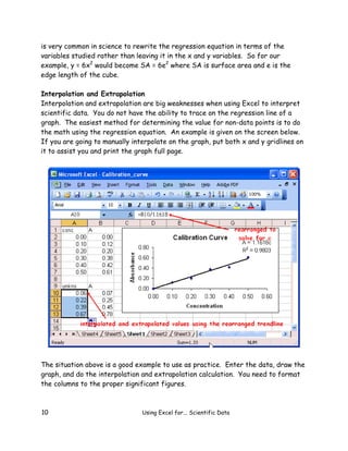
This document provides an overview of using Microsoft Excel to handle, graph, and analyze scientific data. It begins with basics of the Excel interface and entering data. It then demonstrates how to manipulate data through calculations, format cells, and use functions. The document shows how to create scatter plots and add regression lines to graphs. It also discusses interpolation, extrapolation, printing graphs, downloading internet data, and more advanced statistical analyses in Excel.

1. Using Excel for Handling, Graphing,
and Analyzing Scientific Data:
A Resource for Science and
Mathematics Students
Scott A. Sinex
Barbara A. Gage
Department of Physical Sciences and Engineering
Prince George’s Community College
Largo, MD 20774-2199
Spring 2006 version
http://academic.pgcc.edu/psc

2. Acknowledgments
The authors would like to thank
Bridget Bartlebaugh
of the
Computer Information and Office Systems Department

3. TABLE OF CONTENTS
Some Excel Basics
1
Handing and Manipulating Data
3
Displaying an X-Y Data Set as a Scatter Plot
6
Plotting a Regression Equation
8
Interpolation and Extrapolation
10
Printing or Exporting Graphs
11
Downloading Data from the Internet
11
For the More Advanced Statistical Users
12
Using Interactive Excel Spreadsheets or Excelets
14
More Resources
15
An Example of a Printed Chart
16
iii

4. One of the authors on a bad day.
Just hit any key!!!
Where is my graphing calculator?
iv

5. Using Excel for Handling, Graphing, and Analyzing Scientific Data
Excel is a Microsoft computer application called a “spreadsheet.” It is designed to
manage, manipulate, and display data. It has functions appropriate for business
and scientific data sets. Excel is comparable to other spreadsheet applications
such as Quattro Pro by Corel. If you are familiar with the basic layout and
terminology of spreadsheets you can skip this “basics” section or use it for review.
Some Excel Basics
Start Excel and a screen similar to the one below will appear. The main body of
the screen will contain columns labeled with letters (A, B, C...) and rows labeled
with numbers (1, 2, 3...). A cell is a space where numbers, formulas or text can be
entered. Each cell has a designation that gives its location such as F22 (column F,
row 22) or CC115 (column CC, row 115).
Above the main body are two white regions. The left region, the Name box,
indicated which cell or region (such as a chart) is active (selected). The right
region is a Formula bar. Cell contents are displayed here. If you activate a cell
that has a number generated by a formula, the value will appear in the cell but the
Using Excel for... Scientific Data
1

6. formula will appear in the formula bar.
You enter data into a cell by placing the cursor in the cell, clicking, and typing. You
will notice that what you type appears in the cell and in the formula bar. Data is
registered by hitting Enter or using any cursor key to change cell location. If you
need to edit the contents of a cell, click on the cell and then on the formula bar;
you can then change the entry in the cell or in the formula bar. Register as before.
Above the Name box and Formula bar are two rows of icons called the Formatting
and Standard Toolbars. Some of the icons will resemble ones you have seen in
word processors and others are unique to spreadsheets. If you place the cursor on
an icon and wait a few seconds, the name or function of the icon will be displayed.
This tool bar can be customized with additional features you frequently use by
going to View/Toolbars/Customize. Above the tool bar is the Menu bar. Each item
here has a pull-down menu of operations. Note that the menu item that reads Data
on the menu bar (on the graphic above) changes to Chart when you have a chart
active.
If you wish to format a whole column or row of cells, click on the column letter or
row number and the entire column or row will be highlighted. Any change you make,
such as defining the numerical display (under Format) or deleting, will apply to all
of the highlighted cells. If you right-click the letter or number (or any cell) you
will get an abbreviated menu of common operations.
Look at the sample sheet. You will notice that cell D2 contains the formula =A2^3.
If you copy this formula and paste it into D3, Excel will use the value in cell A3
rather than A2 for the calculation. If you paste into cell D4 it will use A4. This is
great if you want to extend a calculation for a whole series of data. However, if
you want to lock in the cell value A2 to be used in all calculations, designate like so:
$A$2. Using the dollar signs will ensure that this cell value will not change.
If you want to designate a series of data values for a calculation such as an
average you can use a shortcut. To designate the values in cells A2 through A6 use
A2:A6. If you want A2 through B6 enter A2:B6.
If you wish to insert or delete a column or row of cells, you can do this through the
menu bar or by right-clicking on the column letter or row number. Excel inserts
2
Using Excel for... Scientific Data

7. columns and rows before or above the highlighted cell. Highlight the column or row
where the insert will occur. Go to Insert on the Menu bar and you will see column
or row displayed as an option. Select that and the insertion will occur. To delete a
row or column, highlight it and go to Edit and select delete. If you use the rightclick option, insert and delete will appear on the menu.
The tabs at the bottom of the screen (Sheet 1...), allow for multiple worksheets to
be used in a file.
Handling and Manipulating Data
Bring up Excel on the computer and a screen like the one below will appear. This is
called a “worksheet” in Excel and since it is active, the word “Data” appears as a
pull-down menu. Many of the toolbar icons are similar to ones used in word
processing programs. Some of the ones more useful in science and math are
labeled below.
The first task is to enter your data into the columns. For ease of graphing, try to
place your independent variable in the first column. You may want to label the
first cell in each column (A1, B1, C1, etc.) with the variable names.
Using Excel for... Scientific Data
3

8. Let’s calculate the surface area and volume of cubes of varying edge length as
outlined below.
1.
Enter the data below into column A: Label length in Al and then start the
data in A2: 1, 2, 3, ... to 10
The second task is to transform or manipulate data.
2.
In B1 type “Area” and in B2 place the formula =6*A2^2 and then press the
enter key. All calculations with a formula must start with an “=” in the cell.
This calculates the surface area of the cube. Grab the lower right hand
corner of the cell and drag down the column. This will copy the formula to
the covered cells. See the screen shot given below.
3.
In C1 type “Volume” and in C2 place the formula =A2^3 and then press the
enter key. This calculates the volume of the cube. Grab the lower right
hand corner of the cell. When the cursor changes form to +, drag the
formula down the column.
4
Using Excel for... Scientific Data

9. The data and two calculated quantities, surface area and volume, should look like
the screen shot above when you are done.
If you right click on the column heading (A, B, C...) you can format the cells for the
number of decimal places or significant figures needed. This is very important
when considering data generated by experimental measurements in science.
Using the Insert Function (fx icon) or from the toolbar,
which lists some common functions as shown to the
right, a vast number of mathematical and statistical
functions can be placed into a formula.
When you select a function, a brief explanation with
syntax is given in the lower part of this screen as seen
below on the Insert Function pop-up screen below.
Further explanation of
the function is available
by clicking on the “Help on
this function.”
This screen shows the
common logarithm
function under Math.
Select the function and
click OK. This will bring
up another pop-up window
with instructions to
follow. Or you can type
the function name in the
formula bar directly.
Remember to follow the syntax. Square root, raise to a power, average, and
standard deviation are a few other examples of available operations.
Using Excel for... Scientific Data
5

10. Displaying an X-Y Data Set as a Scatter Plot
Our third task is to graph the data. This can be done using the Chart Wizard icon
(bar graph) or by finding chart under the insert menu.
1.
Highlight the columns of data to be plotted. Either click on the A and B
column headings or click on the first cell and drag to select the data. The
first column is always treated as the x-variable in Excel.
2.
Click on the icon that looks like a bar
graph. When the Chart Wizard window
appears, select XY (scatter).
The scatter plot is the only graph type
in Excel that will treat the x-axis as a
variable.
All other graph types treat the x-axis
as discrete categories such as days of
the week.
Under chart sub-type select the
unconnected data icon, the first
choice, as this plots only the data points. We rarely use the “connect the
dots” option! Select Finish. A graph should appear on the spreadsheet.
The scatter with data points connected by smooth lines, the second subtype, is used for connecting points on some plots. Excel uses cubic splines to
form a nice smooth curve. In chemistry, an absorption spectrum is a
situation where it is used.
The “connect the dots” with linear segments of the third sub-type is seldom
used especially when plotting experimental data where we are looking for
trends in the data. However, we do use this for plotting properties when
exploring periodic atomic trends in chemistry.
6
Using Excel for... Scientific Data

11. Your graph with the data boxed will appear on the worksheet as shown on the
screen below.
You can add more data to the graph by typing the values into the appropriate cells
and then dragging the lower right-hand corner of the highlighted data. The points
will be plotted and the graph will rescale if needed.
To plot volume against length, select column A by clicking on it, and then press and
hold the control key (Ctrl) and click on column C. Column A and C will be
highlighted (the first column highlighted will be the x-variable.).
3.
Label the axes and decide on the scaling. The chart needs to be active (the
little black squares around the chart), otherwise the word Data appears in
place of Chart. Select Chart from the Menu bar. From the chart menu
select Chart Options. From this window you can assign axes labels (Titles),
legend, and gridlines.
Using Excel for... Scientific Data
7

12. If you click on the x or y-scales on the original graph (not the one in the Chart
Option window), the intervals can be set and the scale can be made logarithmic
instead of linear if required. Font size, color, symbol, etc. can be modified by
clicking on the appropriate chart item and making the change.
Plotting a Regression Equation
Excel refers to a regression
equation as a trendline.
1.
Be sure that the chart is
selected (rather than cells of
data).
2.
Select Chart from the Menu
bar and then select Add
Trendline. The following
window will appear:
3.
Select the Trend/Regression
8
Using Excel for... Scientific Data

13. Type that you think fits the data. If you would like to see the regression
equation displayed on the graph go to Options and be sure the “Display
Equation on Chart” box and the “Display R-squared value on graph” box are
selected. Select OK when finished.
If the equation is displayed on top of the graph just select it by clicking on it (if it
is not already selected) and you can move the equation to another spot. You can
edit the equation to substitute the variables plotted instead of x and y.
The R-squared (R2) is a measure
of the goodness of fit of a
regression to the data. The R2
value times 100 can be
interpreted as the percent of the
y-variable explained by the
variation in the x-variable. A
value of R2 = 1 indicates a perfect
fit of the line to the data.
On the Options window there is a
“Set Intercept =” option. This
controls the y-intercept of a
straight line (b of y = mx + b). For
some situations setting b = 0 is
important in the determination of a more appropriate regression equation (where y
= 0, if x = 0 such as in Beer’s Law).
A final graph might look like this one below. In Excel, the regression equation is
drawn within the range of the data
only. There is a way to extend the
regression line (or extrapolate) by
using the forecast function from the
Options window of Add Trendline,
This graph has a power regression, y
= axb, to fit the data perfectly, since
it was generated by an equation. It
Using Excel for... Scientific Data
9

14. is very common in science to rewrite the regression equation in terms of the
variables studied rather than leaving it in the x and y variables. So for our
example, y = 6x2 would become SA = 6e2 where SA is surface area and e is the
edge length of the cube.
Interpolation and Extrapolation
Interpolation and extrapolation are big weaknesses when using Excel to interpret
scientific data. You do not have the ability to trace on the regression line of a
graph. The easiest method for determining the value for non-data points is to do
the math using the regression equation. An example is given on the screen below.
If you are going to manually interpolate on the graph, put both x and y gridlines on
it to assist you and print the graph full page.
The situation above is a good example to use as practice. Enter the data, draw the
graph, and do the interpolation and extrapolation calculation. You need to format
the columns to the proper significant figures.
10
Using Excel for... Scientific Data

15. Printing or Exporting Graphs
If you select a graph (make it active) and click on print under the File menu, the
graph will be printed full-page. You can select the print area and preview what will
be printed too. The size of the graph can be enlarged by dragging on one of the
corners. Graphs can be moved into word processing programs, such as Word, or
into PowerPoint slides by using the clipboard.
If you right click on a graph on a worksheet and then select Location... from the
menu that pops up, the following window appears.
This allows you to shift the graph to a chart page, which provides a better quality
on printing. A tab labeled “Chart 1” will appear. You can modify the graph as a
chart by clicking on the axes, moving labels, or using the menu choices as before.
An example of a printed chart is given on the last page of this booklet. The
smoothed curve with data points is used there to show the cyclic trend in water
temperature.
Downloading Data from the Internet
Some websites have data that can be downloaded and imported into Excel. If your
web browser saves as an .htm file, use “save as” to select the format as a .txt file.
In Excel, the opened .txt file will come up with a panel “Original Data Type”; select
fixed width and click on next. Then set the break lines for the columns of data
(cursor down file a little in grey box) and click on next. Now the data will load into
columns in the spreadsheet. Save the data as an .xls file.
Using Excel for... Scientific Data
11

16. For the More Advanced Statistical User
Excel has the ability to do some simple statistical analyses. To do this, go to the
Tools menu and select Add-ins... to get the following screen.
Make sure that the Analysis Toolpak and
Analysis Toolpak - VBA are checked.
Then press OK.
Once you have selected the Add-Ins, you
will need to close Excel and then reopen
your file.
Once these have been selected Data Analysis...will appear on the Tools menu.
When selected, Data Analysis... gives the screen below.
12
Using Excel for... Scientific Data

17. When you select an analysis tool another window appears with instructions for that
tool- what data is needed and options for output. The regression analysis (for
linear only) will calculate residuals and plot them.
The residual is the difference between the actual y-value and the y-value obtained
from the regression equation when the appropriate x-value is placed in the
equation. It is the error between the measured y-value and the y-value predicted
by the model or regression equation.
residual = Yactual data value - Yregression equation
Here is the residuals plot for the calibration curve given earlier. This is another
way to judge the goodness of fit of a regression to the data.
Best fit is judged when the residuals are at a minimum, and the plot is random as a
patternless horizontal band (random noise). Even better, the band should take the
shape of a football. It is better to have the residuals at the center of the xvalues be larger than the residuals at the ends of the domain. This has to do with
how much leverage each point has on the regression. A pattern in the residuals
plot, especially near the extremes of the data, indicates that the regression is not
the best fit of the data or there is a better fitting regression. Outliers will stand
out on a residuals plot.
Using Excel for... Scientific Data
13

18. Here is a residuals plot showing a very definite pattern indicating a non-linear
calibration curve even though the R2 = 0.963 for a linear regression of different
absorbance-concentration data.
Using Interactive Excel Spreadsheets or Excelets
There are a number of interactive features in Excel that allow spreadsheets to be
set up to perform a function, such as calculate a result, graph data, or have a graph
respond to a change in a variable (aka, a simulation). These features are shown in
the screen shot below. The yellow input cell, slider, and spinner allow you to adjust
the value of a variable. Cells with a comment box supply information or helpful
hints. The hyperlinks can go to websites or control links from worksheet to
worksheet.
14
Using Excel for... Scientific Data

19. More Resources
Here are some links to further information concerning regression and scatter in
data.
The Best-Fit Straight Line: How do you determine it?
<http://academic.pgcc.edu/~ssinex/regression.xls>
Exploring the Goodness of Fit in Linear Models
<http://www.joma.org/mathDL/4/?pa=content&sa=viewDocument&nodeId=559>
For information on interactive Excel spreadsheets or Excelets, see Developer’s
Guide to Excelets: Dynamic and Interactive Visualization with “Javaless” Applets
or Interactive Excel Spreadsheets
<http://academic.pgcc.edu/~ssinex/excelets>
Copies of this booklet, as well as resources on the graphing calculator, PowerPoint,
Chime Guide, plus others are available at:
http://academic.pgcc.edu/psc
and click on resources for students
Please feel free to email any comments, corrections, or questions!
ssinex@pgcc.edu
bgage@pgcc.edu
Using Excel for... Scientific Data
15

20. 16
Jack Bay on the Patuxent River
1/98 to 6/03
This is a printed chart!
30.00
25.00
Temperature (deg C)
Using Excel for... Scientific Data
20.00
15.00
10.00
5.00
0.00
-5
0
5
10
15
20
25
30
35
Time in months
40
45
50
55
60
65
70