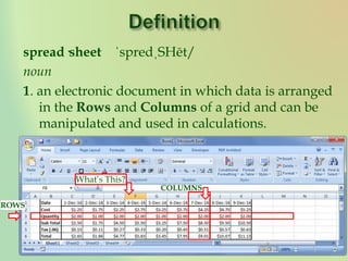
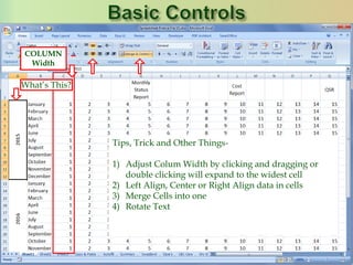
This document provides tips and instructions for using spreadsheets. It begins with definitions of key spreadsheet terminology like cells, rows, and columns. It then gives numerous tips for inputting, formatting, and manipulating data within spreadsheets. These tips include adjusting column widths, inserting and deleting rows and columns, formatting cells, and using basic formulas like SUM. The document demonstrates concepts like copying and pasting formulas while maintaining relative cell references. It also shows functions like autofill and format painter for efficiently applying formats.

1. Cory Steinke

2.  Provide an overview of spreadsheets, their
value in displaying and tracking data, and their
ability to support decision making.
 Provide an understanding of how to input,
manipulate and format data in spreadsheets.

3.  What is a Spreadsheet?
 Various Spreadsheet Programs
 Basic Features
 Cells and Tables
 Managing Your Data
 Basic Settings

4. spread·sheet ˈspredˌSHēt/
noun
1. an electronic document in which data is arranged
in the Rows and Columns of a grid and can be
manipulated and used in calculations.
ROWS
COLUMNS
What’s This?

5. COLUMN
Width
What’s This?
Tips, Trick and Other Things-
1) Adjust Colum Width by clicking and dragging or
double clicking will expand to the widest cell
2) Left Align, Center or Right Align data in cells
3) Merge Cells into one
4) Rotate Text

6. Tips, Trick and Other Things-
1) Hide Rows or Columns to only see your work area (Click & Drag or Double Click)
2) Adjust Column Width or Row Height (Click & Drag or Double Click)
3) Insert Rows or Columns using Ribbon or Right Click and Insert
function for entire row or selected cells allowing “Shifting of cells.”
4) Delete Rows or Columns using Ribbon or Right Click & Delete.
5) Use View Dividers to display Headers.
6) Use Alt+Enter to force Return within a cell.
7) Format Cells: Cntl+1 or...
Checkout Spreadsheet Practice File V1.xls /Sheet1

7.  MS Excel (primary) for iPad, Mac, IBM
 Numbers for Apple/Mac
 OpenOffice Spreadsheets
 iSpreadsheet
 Google Sheets
 Numerous Others!

8. What’s This?
=SUM(C7:C8)
Select this Cell
Notice
These Cells Are Added Together and displayed in D8!
Note Cell
Properties
Displayed
For Selected
Cells
Note that a “threshold” has been exceeded and
“Conditional Formatting” changes the cell
Properties to cause it to turn Red.

9. Can be shared for collaboration via network/cloud

10. What Cell is Selected?What kind of data in in the
Cell?
Let’s Move To the Cell on
the Right!
What kind of data in in the
Cell?
Let’s Move To the Cell on
the Right!
What kind of data in in the
Cell?
Note that all the progressive dates are simple
formulas!
What kind of data in in the
Cell?
How does this Formula work.... And note how
it progresses to the cells to the right!
Note that this is a simple number, with no
digits past the decimal. We’ll look at how to
format later.
See how this formula works!
So imagine what formula you could place in
the cell below (D5) to compute your 6% tax!
Is this the formula you imagined?
What is the formula in the cell below (D6)?
Is this the formula you imagined?
Can it be done another way?
Checkout Spreadsheet Practice File V1.xls /Sheet2
Are there other ways to get the cell to result
in the same end state or total?
An alternative might look like:
=SUM(D4+D5)

11. Type or Input Data
In order to input data in Excel click on any of the empty cells and type. You can type
numbers, words or a mixture in these cells. To navigate you can use the mouse as
well as the keyboard Arrow keys. When you type something in Excel you can press
“enter” or “tab” to accept the input data and the cursor will move to the next cell. If
you want to remain on the same call then press “ctrl + enter” and your cursor will
remain on the same cell and you can now change formatting like Bold, Center text, or
change cell formatting like background color, etc.
Many people like to type in all the data, then
come back and work on the formatting.
Others may format as they go.

12. Navigation - Press Ctrl + Home or Ctrl + End
Since Excel has a lot of rows or columns it can be time consuming to scroll all the way
down or across to go to the last cell. If you press the “Ctrl + end” key then you will be
taken to the last cell. In order to come back to the first cell you can press “ctrl+ home”

13. View the Empty Cell
There are times when the width and the height of a cell is less and a long word does
not fit in just one cell. When you enter the long word it overlaps the next empty cell
and displays the entire text. It appears that the cell next to it also contains this text
data but that is not the case. When you click on the “cell” the formula bar shows that
the cell has nothing in it. If you enter any data in it then the text which was
displayed, from the first cell will be covered up with the new data that is visible.
Now that we placed text in Cell B1, it covers
up the extended text in A1.
What can we do to display both cells
completely?
Can you manually and automatically adjust
Cell Width or Height?
Click on Cell B1 and enter the Text:
“This is a Test”

14. Copy and Pasting Formula’s.
When you Copy and Paste a Formula the Cells remain “Relational”.
This Cell:
is using
this
Formula
This Cell...
is multiplied
by this one
The Formula
in this cell is
the same
This Cell:
is using
this
Formula
Or Could
be...
this Formula
These Cells
simply total
those cells
from above.
Note that $D$9
is Referencing
This Cell!
Note that the below Row provides Column References for this example

15. Copy and Pasting Formula’s.
When you Copy and Paste a Formula the Cells remain “Relational”.
Select the
Cells in
Column C
...Copy
& Paste in
Column D
Note that the below Row provides Column References for this example

16. Copy and Pasting Formula’s.
When you Copy and Paste a Formula the Cells remain “Relational”.
Notice how both sets of Cells when Pasted provide
a “Relational” reference to the previous Cell.
This will continually “progress” as far as you paste or
Autofill cells.
Can you see how these Cells Differ?
The Cell on the left has the 6% tax embedded while the Cell on
the Right uses the $ to point to a “Single Specific Cell” and
progressive cells will still point to this specific cell.
Note that the below Row provides Column References for this example
Notice how all pasted Cells “progress” the formula’s?
Can you see the advantage of using a “Absolute” reference
with the $ instead of embedding the 6% into the formula and
then using the “Relative” reference?

17. Use ‘Autofill’ Option
Suppose you have a sheet with many rows and you want to apply the same formula
to each of these rows. Instead of dragging the formula all the way down, you can
simply use the “Autofill” function. Simply double click towards the lower right side
of the cell in which the formula is, and it will be copied all the way down.
Alternatively you can also press “Ctrl + .” on your keyboard for the same result. The
Autofill Options Button will display after pasting all available cells.
Note Standard
Mouse Cursor
Note Cursor
Changes When
Moved To Lower Right
Corner of selected
Cell
Double Click on
Lower Right Corner
Of Selected Cell

18. Format Painter:
Go to the Copy & Paste Tab then scroll to the right.
Select a group of Cells, like those in Column K, then Select the Format Painter Icon
to copy the formatting and apply it to any adjacent set of cells.

19. View the Paste Options
Copying and Pasting in Excel is just like any other MS Office program. However,
when you paste the data, there are a few options which are very helpful. When you
copy the data and “right click” on the cell where you want to paste it, select “Paste
Special” (2007) a few pasting options appear in front of you. You can choose from
any one of them depending on the requirement you have at the time.
NOTE: When copying and pasting a cell that contains a function the pasted function will be
“relative” to the location of the pasted cell.
2007
2010

20. All: paste all data in the cell selection (formulas, formatting, etc.). this is what happens when you paste normally.
Formulas to paste all the text, numbers, and formulas in the current cell selection without their formatting.
Values to convert formulas in the current cell selection to their calculated values.
Formats to paste only the formatting from the current cell selection, without the cell entries.
Comments to paste only the notes that you attach to their cells (kinda like electronic self-stick notes).
Validation: paste only data validation rules in the cell range that you set up with the Data Validation command.
All Using Source Theme to paste all the information plus the cell styles applied to the cells.
All Except Borders to paste all the stuff in the cell selection without copying any borders you use there.
Column Widths to apply the column widths of the cells copied to the Clipboard to the columns where pasted.
Formulas and Number Formats to include the number formats assigned to the pasted values and formulas.
Values and Number Formats to convert formulas to their calculated values and include the number formats you
assigned to all the copied or cut values. You can also perform some math when you paste based on the value(s)
in the copied or cut cell(s) and the value in the target cell(s):
None: Excel performs no operation between the data entries you cut or copy to the Clipboard and the data entries
in the cell range where you paste. This is the default setting.
Add: Excel adds the values you cut or copy to the Clipboard to the values in the cell range where you paste.
Subtract: Excel subtracts the values you copy to the Clipboard from the values in the cell range where pasted.
Multiply: Excel multiplies the data you copy to the Clipboard by the data entries in the cell range where pasted.
Divide: Excel divides the data you copy to the Clipboard by the data entries in the cell range where you paste.
Selecting the Skip Blanks check box tells Excel only to paste from those cells that aren't empty.
Selecting the Transpose check box changes the orientation of the pasted entries. For example, if the original cells’
entries run down a single column of the worksheet, the transposed pasted entries will run across a single row.
Clicking the Paste Link button establishes a link between the copies you’re pasting and the original entries. That
way, changes to the original cells automatically update in the pasted copies.

21. Paste data as an Image/Picture
Excel allows you to copy the data and paste it as an image. First copy the data (select
the cells) then click on the small pull down arrow at the bottom center of the Paste
button which is situated on the top left corner of the Home Ribbon. A drop down
menu will appear and you can choose “Picture,” then “paste as picture.”
Date 1-Dec-14
Cost $1.25
Quantity 2
Sub Total $2.50
Tax (.06) $0.15
Total $2.65
Percent 13.00%
Fraction 1/4
Time 1:30 AM

22. Paste data Into Other Programs?
Excel allows you to copy and paste data into any program, HOWEVER, do you
merely want to post the data for “display” or do you want the “functions” of Excel to
exist like formula’s that will calculate new input data and then display?
If you Merely “Copy” then “Paste” you will get a Table of the Data Values.
The Table of working functions will become mere numbers.

23. 12.50
1,000
13,500.00
2.00
2.50
1.10
0.80
1.20
7.60
7,600.00
5.90
5,900.00
1,200.00
500.00
150.00
800.00
750.00
3,400.00
2,500.00

24. Paste data Into Other Programs?
To Paste the data with full Excel Functionality you must past it as a Microsoft Office
Graphic Object. (Some programs list it as an Excel Object)
1) Highlight and “Copy” the data from Excel.”.1) Highlight and “Copy” the data from Excel.
2) Launch PowerPoint and select “Paste Special”.

25. Breakeven Analysis
EXAMPLE
Amounts shown in U.S. dollars
Sales
Sales price per unit 13.50
Sales volume per period (units) 1,000
Total Sales 13,500.00
Variable Costs
Commission per unit 2.00
Direct material per unit 2.50
Shipping per unit 1.10
Supplies per unit 0.80
Other variable costs per unit 1.20
Variable costs per unit 7.60
Total Variable Costs 7,600.00
Unit contribution margin 5.90
Gross Margin 5,900.00
Fixed Costs Per Period
Administrative costs 1,200.00
Insurance 500.00
Property tax 150.00
Rent 800.00
Other fixed costs 750.00
Total Fixed Costs per period 3,400.00
Net Profit (Loss) 2,500.00
Results:
Breakeven Point (units): 576
Sales volume analysis:
Sales volume per period (units) 0 100 200 300 400 500 600 700 800 900 1,000
Sales price per unit 13.50 13.50 13.50 13.50 13.50 13.50 13.50 13.50 13.50 13.50 13.50
Fixed costs per period 3,400.00 3,400.00 3,400.00 3,400.00 3,400.00 3,400.00 3,400.00 3,400.00 3,400.00 3,400.00 3,400.00
Variable costs 0.00 760.00 1,520.00 2,280.00 3,040.00 3,800.00 4,560.00 5,320.00 6,080.00 6,840.00 7,600.00
Total costs 3,400.00 4,160.00 4,920.00 5,680.00 6,440.00 7,200.00 7,960.00 8,720.00 9,480.00 10,240.00 11,000.00
Total sales 0.00 1,350.00 2,700.00 4,050.00 5,400.00 6,750.00 8,100.00 9,450.00 10,800.00 12,150.00 13,500.00
Net profit (loss) (3,400.00) (2,810.00) (2,220.00) (1,630.00) (1,040.00) (450.00) 140.00 730.00 1,320.00 1,910.00 2,500.00
7.60 ,
56%
5.90 ,
44%
Unit Contribution Margin
Variable costs per unit
Unit contribution margin
2.00 , 26%
2.50 , 33%
1.10 , 14%
0.80 , 11%
1.20 , 16%
Variable Costs Per Unit
Commission per unit
Direct material per unit
Shipping per unit
Supplies per unit
Other variable costs per unit

26. Top 10 Formulas
1. SUM
Formula: =SUM(5, 5) or =SUM(A1, B1) or =SUM(A1:B5)
The SUM formula does exactly what you would expect. It allows you to add 2 or
more numbers together. You can use cell references as well in this formula.
The above shows you different examples. You can have numbers in there separated
by commas and it will add them together for you, you can have cell references and as
long as there are numbers in those cells it will add them together for you, or you can
have a range of cells with a colon in between the 2 cells, and it will add the numbers
in all the cells in the range.
Hold down CNTRL and select additional
cells then hit Tab or Enter.
Click on the Cell we just entered the
formula into.
Click in the Formula Bar then notice that it
highlights the cells used in the formula.
Click and Drag the Green Highlighted Cell
and Drag it down to a new location.
Then hit Tab or Enter.

27. Top 10 Formulas
1. SUM
Formula: =SUM(5, 5) or =SUM(A1, B1) or =SUM(A1:B5)
Selecting Multiple Cells
Can you double click on the Black,
Lower Right Corner of the selected Cell to
Autofill?
Select a Cell from the E Column.
Select the Sum Icon.
Click and Drag to select a Group of Cells.
• Notice the “Included” Cells are A3:D3
• This can be used to select any Group of
adjacent Cells.
• You can Also Individually Select Cells by
holding down the Cntl Key and selecting
the desired Cells.

28. Top 10 Formulas
2. COUNT
Formula: =COUNT(A1:A10)
The count formula counts the number of cells in a range that have numbers in them.
This formula only works with numbers.

29. Top 10 Formulas
3. COUNTA
Formula: =COUNTA(A1:A10)
Counts the number of non-empty cells in a range. It will count cells that have
numbers and/or any other characters in them.
The COUNTA Formula works with all data types.

30. Top 10 Formulas
4. LEN
Formula: =LEN(A1)
The LEN formula counts the number of characters in a cell. Be careful though! This
includes spaces.
Notice the difference in the formula results:
10 characters without spaces in between the words,
12 characters with spaces between the words.

31. Top 10 Formulas
5. TRIM
Formula: =TRIM(A1)
Gets rid of any space in a cell, except for single spaces between words. I’ve found this
formula to be extremely useful because I’ve often run into situations where you pull
data from a database and for some reason extra spaces are put in behind or in front of
legitimate data. This can wreak havoc if you are trying to compare using IF
statements or VLOOKUP’s.
I added in an extra space behind “I Love Excel”.
The TRIM formula removes that extra space. See the
character count difference with or without the TRIM formula.

32. Top 10 Formulas
6. RIGHT, LEFT, MID
Formulas: = RIGHT(text, number of characters), =LEFT(text, number of characters),
=MID(text, start number, number of characters).
(Note: In all of these formulas, wherever it says “text” you can use a cell reference as
well)
Top 10 Formulas
6. RIGHT, LEFT, MID
These formulas return the specified number of characters from a text string. RIGHT
gives you the number of characters from the right of the text string, LEFT gives you
the number of characters from the left, and MID gives you the specified number of
characters from the middle of the word. You tell the MID formula where to start with
the start_number and then it grabs the specified number of characters to the right of
the start_number.
I used the LEFT formula to get the first word.
I had it look in cell A1 and grab only the 1st character from the left.
I used the MID formula to get the middle word.
I had it look in cell A1, start at character 3, and grab 5 characters after that.
I used the RIGHT formula to get the last word.
I had it look at cell A1 and grab the first 6 characters from the right.

33. Top 10 Formulas
7 VLOOKUP
Formula: =VLOOKUP(lookup_value, table_array, col_index_num, range_lookup)
This Formula looks for a value in the leftmost column of a table, and then returns a
value in the same row from a column you specify.
Basically, you define a value (the lookup_value) for the formula to look for. It looks
for this value in the leftmost column of a table (the table_array).
If it finds a match of the “lookup_value” in the left column of the “table_array” it will
return the value in the column you specify using the “index_num”. The “index_num”
is relative to the left most column.
Exact Match
=VLOOKUP(B22,...)
=VLOOKUP(B23,...)
Top 10 Formulas
7 VLOOKUP
Formula: =VLOOKUP(lookup_value, table_array, col_index_num, range_lookup)
This Formula looks for a value in the leftmost column of a table, and then returns a
value in the same row from a column you specify.

34. Top 10 Formulas
8 IF Statements
Formula: =IF(logical_statement, return this if logical statement is true, return this if
logical statement is false)
When you’re doing an analysis of a lot of data in Excel there are a lot of scenarios you
could be trying to discover and the data has to react differently based on a different
situation.
Let’s say our salesperson has a quota to meet. You used VLOOKUP to put the
revenue next to the name. Now you can use an IF statement that says: “IF the
salesperson met their quota, say “Met quota”, if not say “Did not meet quota”
Cell E3
Imagine Column C is linked to a current sales database. This could be a simple report.

35. Top 10 Formulas
9 SUMIF, COUNTIF, AVERAGEIF
Formulas: =SUMIF(range, criteria, sum_range), =COUNTIF(range, criteria),
=AVERAGEIF(range, criteria, average_range)
These formulas all do their respective functions IF the criteria are met. There are also
the formulas: SUMIFS, COUNTIFS, AVERAGEIFS where they will do their respective
functions based on multiple criteria you give the formula.
742,733.57

36. Top 10 Formulas
10 CONCATENATE
A fancy word for combining data in 2 (or more) different cells into one cell.
This can be done with the Concatenate excel formula or it can be done by simply
putting the & symbol in between the two cells. If I have “Steve” in cell A1 and
“Quatrani” in cell B1 I could put this formula: =A1&” “&B1 and it would provide
“Steve Quatrani” (The “ “ puts a space in between what you are combining with the
&).
I can use =concatenate(A1, “ “, B1) and it will give the same thing: “Steve Quatrani”

39. Breakeven Analysis
EXAMPLE
Amounts shown in U.S. dollars
Sales
Sales price per unit 13.50
Sales volume per period (units) 1,000
Total Sales 13,500.00
Variable Costs
Commission per unit 2.00
Direct material per unit 2.50
Shipping per unit 1.10
Supplies per unit 0.80
Other variable costs per unit 1.20
Variable costs per unit 7.60
Total Variable Costs 7,600.00
Unit contribution margin 5.90
Gross Margin 5,900.00
Fixed Costs Per Period
Administrative costs 1,200.00
Insurance 500.00
Property tax 150.00
Rent 800.00
Other fixed costs 750.00
Total Fixed Costs per period 3,400.00
Net Profit (Loss) 2,500.00
Results:
Breakeven Point (units): 576
Sales volume analysis:
Sales volume per period (units) 0 100 200 300 400 500 600 700 800 900 1,000
Sales price per unit 13.50 13.50 13.50 13.50 13.50 13.50 13.50 13.50 13.50 13.50 13.50
Fixed costs per period 3,400.00 3,400.00 3,400.00 3,400.00 3,400.00 3,400.00 3,400.00 3,400.00 3,400.00 3,400.00 3,400.00
Variable costs 0.00 760.00 1,520.00 2,280.00 3,040.00 3,800.00 4,560.00 5,320.00 6,080.00 6,840.00 7,600.00
Total costs 3,400.00 4,160.00 4,920.00 5,680.00 6,440.00 7,200.00 7,960.00 8,720.00 9,480.00 10,240.00 11,000.00
Total sales 0.00 1,350.00 2,700.00 4,050.00 5,400.00 6,750.00 8,100.00 9,450.00 10,800.00 12,150.00 13,500.00
Net profit (loss) (3,400.00) (2,810.00) (2,220.00) (1,630.00) (1,040.00) (450.00) 140.00 730.00 1,320.00 1,910.00 2,500.00
7.60 ,
56%
5.90 ,
44%
Unit Contribution Margin
Variable costs per unit
Unit contribution margin
2.00 , 26%
2.50 , 33%
1.10 , 14%
0.80 , 11%
1.20 , 16%
Variable Costs Per Unit
Commission per unit
Direct material per unit
Shipping per unit
Supplies per unit
Other variable costs per unit

42. Summary Tab -
1) Functions for Averaging Columns
2) Display of extended data adjusting View for Headers
3) Data Formats (Percents, digits past decimal, Fonts, etc.)
4) Summary of Data from other “Individual” Worksheets (Autosum)
5) Conditional Formatting
6) Sorting Data by Columns

43. Summary Tab -
1) Review overall Wookbook
2) Understand relationship between Worksheets
3) Check each Red Highlighted Cell For:
1) Accuracy of Data from other “Individual” Worksheets (Autosum)
2) Data Format is Viable/Feasible
3) Relational to what is needed
4) Report Errors

44. THE TEST-
1. Financial Summary Cells:
2) Revenue Cells:
3) Personnel Cells:
4) Compensation Cells:
 B6
 B7
 B19
 B28
 B8
 B9
 B29
 B30
 H5
 I5
 H6
 I6
 H7
 B4
 B5
 B24
 B25
 B7
 B8
 C25
 D32
 B9
 H9
 B14
 B24
 B12
 B13
 B28
 D36