2. tensor algebra jan 2013

Tensor Algebra
Tensors as Linear Mappings

Second Order Tensor

A second Order Tensor 𝑻 is a linear mapping from a
vector space to itself. Given 𝒖 ∈ V the mapping,
𝑻: V → V
states that ∃ 𝒘 ∈ V such that,
𝑻 𝒖 = 𝒘.
Every other definition of a second order tensor can be
derived from this simple definition. The tensor
character of an object can be established by observing
its action on a vector.

Department of Systems Engineering, University of Lagos 2 oafak@unilag.edu.ng 12/30/2012

Linearity

 The mapping is linear. This means that if we have two
runs of the process, we first input 𝒖 and later input 𝐯.
The outcomes 𝑻(𝒖) and 𝑻(𝐯), added would have
been the same as if we had added the inputs 𝒖 and
𝐯 first and supplied the sum of the vectors as input.
More compactly, this means,
𝑻 𝒖 + 𝐯 = 𝑻(𝒖) + 𝑻(𝐯)


Linearity
Linearity further means that, for any scalar 𝛼 and tensor 𝑻
𝑻 𝛼𝒖 = 𝛼𝑻 𝒖
The two properties can be added so that, given 𝛼, 𝛽 ∈ R, and
𝒖, 𝐯 ∈ V, then
𝑻 𝛼𝒖 + 𝛽𝐯 = 𝛼𝑻 𝒖 + 𝛽𝑻 𝐯
Since we can think of a tensor as a process that takes an
input and produces an output, two tensors are equal only if
they produce the same outputs when supplied with the same
input. The sum of two tensors is the tensor that will give an
output which will be the sum of the outputs of the two
tensors when each is given that input.


Vector Space

In general, 𝛼, 𝛽 ∈ R , 𝒖, 𝐯 ∈ V and 𝑺, 𝑻 ∈ T
𝛼𝑺𝒖 + 𝛽𝑻𝒖 = (𝛼𝑺 + 𝛽𝑻)𝒖

With the definition above, the set of tensors constitute
a vector space with its rules of addition and
multiplication by a scalar. It will become obvious later
that it also constitutes a Euclidean vector space with its
own rule of the inner product.


Special Tensors

Notation.
It is customary to write the tensor mapping without the
parentheses. Hence, we can write,
𝑻𝒖 ≡ 𝑻(𝒖)
For the mapping by the tensor 𝑻 on the vector variable
and dispense with the parentheses unless when
needed.


Zero Tensor or Annihilator

The annihilator 𝑶 is defined as the tensor that maps all
vectors to the zero vector, 𝒐:
𝑶𝑢 = 𝒐, ∀𝒖 ∈ V


The Identity

The identity tensor 𝟏 is the tensor that leaves every
vector unaltered. ∀𝒖 ∈ V ,
𝟏𝒖 = 𝒖
Furthermore, ∀𝛼 ∈ R , the tensor, 𝛼𝟏 is called a
spherical tensor.
The identity tensor induces the concept of an inverse of
a tensor. Given the fact that if 𝑻 ∈ T and 𝒖 ∈ V , the
mapping 𝒘 ≡ 𝑻𝒖 produces a vector.


The Inverse

Consider a linear mapping that, operating on 𝒘,
produces our original argument, 𝒖, if we can find it:
𝒀𝒘 = 𝒖
As a linear mapping, operating on a vector, clearly, 𝒀 is a
tensor. It is called the inverse of 𝑻 because,
𝒀𝒘 = 𝒀𝑻𝒖 = 𝒖
So that the composition 𝒀𝑻 = 𝟏, the identity mapping.
For this reason, we write,
𝒀 = 𝑻−1


Inverse

It is easy to show that if 𝒀𝑻 = 𝟏, then 𝑻𝒀 = 𝒀𝑻 = 𝟏.
 HW: Show this.
The set of invertible sets is closed under composition. It
is also closed under inversion. It forms a group with the
identity tensor as the group’s neutral element


Transposition of Tensors

Given 𝒘, 𝐯 ∈ V , The tensor 𝑨T satisfying
𝒘 ⋅ 𝑨T 𝐯 = 𝐯 ⋅ (𝑨𝒘)
Is called the transpose of 𝐴.
A tensor indistinguishable from its transpose is said to
be symmetric.


Invariants

There are certain mappings from the space of tensors
to the real space. Such mappings are called Invariants of
the Tensor. Three of these, called Principal invariants
play key roles in the application of tensors to continuum
mechanics. We shall define them shortly.
The definition given here is free of any association with
a coordinate system. It is a good practice to derive any
other definitions from these fundamental ones:


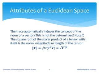
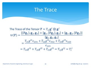
The Trace
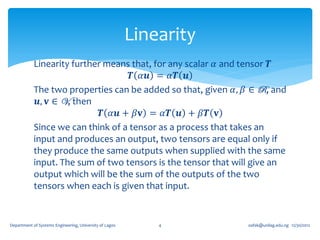
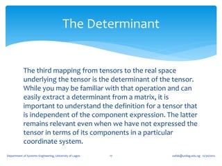
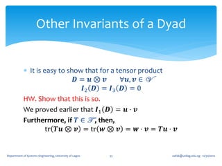
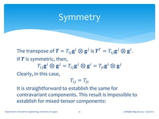
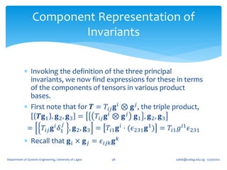
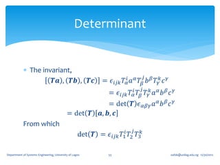
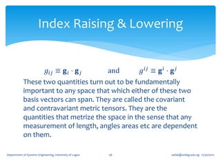
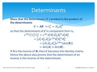
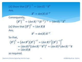
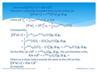
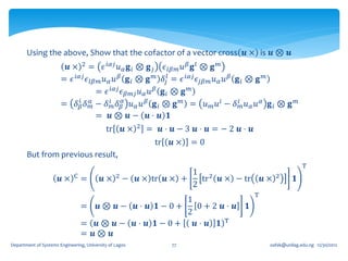
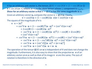
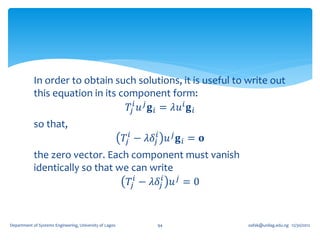
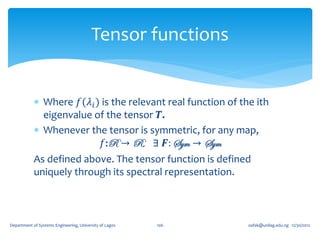
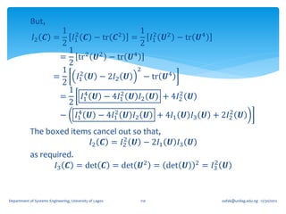
If we write
𝐚, 𝐛, 𝐜 ≡ 𝐚 ⋅ 𝐛 × 𝐜
 where 𝐚, 𝐛, and 𝐜 are arbitrary vectors.
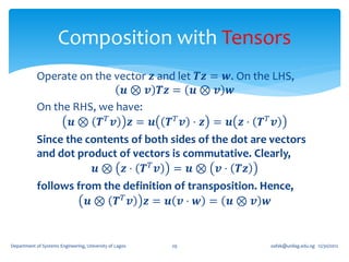
For any second order tensor 𝑻, and linearly
independent 𝐚, 𝐛, and 𝐜, the linear mapping 𝐼1 : T → R
𝑻𝐚, 𝐛, 𝐜 + 𝐚, 𝑻𝐛, 𝐜 + [𝐚, 𝐛, 𝑻𝐜]
𝐼1 𝑻 ≡ tr 𝑻 =
[𝐚, 𝐛, 𝐜]
Is independent of the choice of the basis vectors 𝐚, 𝐛,
and 𝐜. It is called the First Principal Invariant of 𝑻 or
Trace of 𝑻 ≡ tr 𝑻 ≡ 𝐼1 (𝑻)


The Trace

The trace is a linear mapping. It is easily shown that
𝛼, 𝛽 ∈ R , and 𝑺, 𝑻 ∈ T
tr 𝛼𝑺 + 𝛽𝑻 = 𝛼tr 𝑺 + 𝛽tr(𝑻)
HW. Show this by appealing to the linearity of the
vector space.
While the trace of a tensor is linear, the other two
principal invariants are nonlinear. WE now proceed to
define them


Square of the trace

The second principal invariant 𝐼2 𝑺 is related to the
trace. In fact, you may come across books that define it
so. However, the most common definition is that
1 2
𝐼2 𝑺 = 𝐼1 𝑺 − 𝐼1 (𝑺2 )
2
Independently of the trace, we can also define the
second principal invariant as,


Second Principal Invariant

The Second Principal Invariant, 𝐼2 𝑻 , using the same
notation as above is
𝑻𝒂 , 𝑻𝒃 , 𝒄 + 𝒂, 𝑻𝒃 , 𝑻𝒄 + 𝑻𝒂 , 𝒃, 𝑻𝒄
𝒂, 𝒃, 𝒄
1 2
= tr 𝑻 − tr 𝑻2
2
that is half the square of trace minus the trace of the
square of 𝑻 which is the second principal invariant.
 This quantity remains unchanged for any arbitrary
selection of basis vectors 𝒂, 𝒃 and 𝒄.

The Determinant

The third mapping from tensors to the real space
underlying the tensor is the determinant of the tensor.
While you may be familiar with that operation and can
easily extract a determinant from a matrix, it is
important to understand the definition for a tensor that
is independent of the component expression. The latter
remains relevant even when we have not expressed the
tensor in terms of its components in a particular
coordinate system.

The Determinant

As before, For any second order tensor 𝑻, and any
linearly independent vectors 𝐚, 𝐛, and 𝐜,
 The determinant of the tensor 𝑻,
𝑻𝒂 , 𝑻𝒃 , 𝑻𝒄
det 𝑻 =
𝒂, 𝒃, 𝒄
(In the special case when the basis vectors are
orthonormal, the denominator is unity)


Other Principal Invariants

 It is good to note that there are other principal
invariants that can be defined. The ones we defined
here are the ones you are most likely to find in other
texts.
 An invariant is a scalar derived from a tensor that
remains unchanged in any coordinate system.
Mathematically, it is a mapping from the tensor space
to the real space. Or simply a scalar valued function
of the tensor.


Inner Product of Tensors

The trace provides a simple way to define the inner
product of two second-order tensors. Given 𝑺, 𝑻 ∈ T
The trace,
tr 𝑺 𝑇 𝑻 = tr(𝑺𝑻 𝑇 )
Is a scalar, independent of the coordinate system
chosen to represent the tensors. This is defined as the
inner or scalar product of the tensors 𝑺 and 𝑻. That is,
𝑺: 𝑻 ≡ tr 𝑺 𝑇 𝑻 = tr(𝑺𝑻 𝑇 )


Attributes of a Euclidean Space

The trace automatically induces the concept of the
norm of a vector (This is not the determinant! Note!!)
The square root of the scalar product of a tensor with
itself is the norm, magnitude or length of the tensor:
𝑻 = tr(𝑻 𝑇 𝑻) = 𝑻: 𝑻


Distance and angles

Furthermore, the distance between two tensors as well
as the angle they contain are defined. The scalar
distance 𝑑(𝑺, 𝑻)between tensors 𝑺 and 𝑻 :
𝑑 𝑺, 𝑻 = 𝑺 − 𝑻 = 𝑻 − 𝑺
And the angle 𝜃(𝑺, 𝑻),
−1
𝑺: 𝑻
𝜃 = cos
𝑺 𝑻


The Tensor Product

A product mapping from two vector spaces to T is
defined as the tensor product. It has the following
properties:
"⊗": V × V → T
𝒖 ⊗ 𝒗 𝒘 = (𝒗 ⋅ 𝒘)𝒖
It is an ordered pair of vectors. It acts on any other
vector by creating a new vector in the direction of its
first vector as shown above. This product of two
vectors is called a tensor product or a simple dyad.


Dyad Properties
It is very easily shown that the transposition of dyad is
simply a reversal of its order. (HW. Show this).
The tensor product is linear in its two factors.
Based on the obvious fact that for any tensor 𝑻 and
𝒖, 𝒗, 𝒘 ∈ V , 𝑻 𝒖 ⊗ 𝒗 𝒘 = 𝑻𝒖 𝒗 ⋅ 𝒘 = 𝑻𝒖 ⊗ 𝒗 𝒘
It is clear that
𝑻 𝒖 ⊗ 𝒗 = 𝑻𝒖 ⊗ 𝒗
Show this neatly by operating either side on a vector
Furthermore, the contraction,
𝒖⊗ 𝒗 𝑻= 𝒖⊗ 𝑻𝑇 𝒗
A fact that can be established by operating each side
on the same vector.

Transpose of a Dyad
Recall that for 𝒘, 𝐯 ∈ V , The tensor 𝑨T satisfying
𝒘 ⋅ 𝑨T 𝐯 = 𝐯 ⋅ (𝑨𝒘)
Is called the transpose of 𝑨. Now let 𝑨 = 𝒂 ⊗ 𝒃 a dyad.
𝐯 ⋅ 𝑨𝒘 =
= 𝐯⋅ 𝒂⊗ 𝒃 𝒘 = 𝐯⋅ 𝒂 𝒃⋅ 𝒘
= 𝐯⋅ 𝒂 𝒃⋅ 𝒘 = 𝒘⋅ 𝒃 𝐯⋅ 𝒂
= 𝒘⋅ 𝒃⊗ 𝒂 𝐯
So that 𝒂 ⊗ 𝒃 T = 𝒃 ⊗ 𝒂
Showing that the transpose of a dyad is simply a
reversal of its factors.


If 𝐧 is the unit normal to a given plane, show that the
tensor 𝐓 ≡ 𝟏 − 𝐧 ⊗ 𝐧 is such that 𝐓𝐮 is the projection
of the vector 𝐮 to the plane in question.
Consider the fact that
𝐓 ⋅ 𝐮 = 𝟏𝐮 − 𝐧 ⋅ 𝐮 𝐧 = 𝐮 − 𝐧 ⋅ 𝐮 𝐧
The above vector equation shows that 𝐓𝐮 is what
remains after we have subtracted the projection
𝐧 ⋅ 𝐮 𝐧 onto the normal. Obviously, this is the
projection to the plane itself. 𝐓 as we shall see later is
called a tensor projector.


Substitution Operation
Consider a contravariant vector component 𝑎 𝑘 let us take a
product of this with the Kronecker Delta:
𝛿 𝑗𝑖 𝑎 𝑘
which gives us a third-order object. Let us now perform a
contraction across (by taking the superscript index from 𝐴 𝑘
and the subscript from 𝛿 𝑗𝑖 ) to arrive at,
 𝑑 𝑖 = 𝛿 𝑗𝑖 𝑎 𝑗
 Observe that the only free index remaining is the
superscript 𝑖 as the other indices have been contracted (it
is consequently a summation index) out in the implied
summation. Let us now expand the RHS above, we find,


Substitution
𝑑 𝑖 = 𝛿 𝑗𝑖 𝑎 𝑗 = 𝛿1𝑖 𝑎1 + 𝛿2 𝑎2 + 𝛿3 𝑎3
𝑖 𝑖

Note the following cases:
 if 𝑖 = 1, we have 𝑑1 = 𝑎1 , if 𝑖 = 2, we have 𝑑 2 = 𝑎2 if
𝑖 = 3, we have 𝑑 3 = 𝑎3 . This leads us to conclude
therefore that the contraction, 𝛿 𝑗𝑖 𝑎 𝑗 = 𝑎 𝑖 . Indicating
that that the Kronecker Delta, in a contraction,
merely substitutes its own other symbol for the
symbol on the vector 𝑎 𝑗 it was contracted with. This
fact, that the Kronecker Delta does this in general
earned it the alias of “Substitution Operator”.


Composition with Tensors
Operate on the vector 𝒛 and let 𝑻𝒛 = 𝒘. On the LHS,
𝒖 ⊗ 𝒗 𝑻𝒛 = 𝒖 ⊗ 𝒗 𝒘
On the RHS, we have:
𝒖⊗ 𝑻𝑇 𝒗 𝒛= 𝒖 𝑻𝑇 𝒗 ⋅ 𝒛 = 𝒖 𝒛⋅ 𝑻𝑇 𝒗
Since the contents of both sides of the dot are vectors
and dot product of vectors is commutative. Clearly,
𝒖 ⊗ 𝒛 ⋅ 𝑻 𝑇 𝒗 = 𝒖 ⊗ 𝒗 ⋅ 𝑻𝒛
follows from the definition of transposition. Hence,
𝒖⊗ 𝑻𝑇 𝒗 𝒛= 𝒖 𝒗⋅ 𝒘 = 𝒖⊗ 𝒗 𝒘


Dyad on Dyad Composition
For 𝒖, 𝒗, 𝒘, 𝒙 ∈ V , We can show that the dyad
composition,
𝒖⊗ 𝒗 𝒘⊗ 𝒙 = 𝒖⊗ 𝒙 𝒗⋅ 𝒘
Again, the proof is to show that both sides produce the
same result when they act on the same vector. Let
𝒚 ∈ V , then the LHS on 𝒚 yields:
𝒖 ⊗ 𝒗 𝒘 ⊗ 𝒙 𝒚 = 𝒖 ⊗ 𝒗 𝒘(𝒙 ⋅ 𝒚)
= 𝒖 𝒗 ⋅ 𝒘 (𝒙 ⋅ 𝒚)
Which is obviously the result from the RHS also.
This therefore makes it straightforward to contract
dyads by breaking and joining as seen above.

Trace of a Dyad

Show that the trace of the tensor product 𝐮 ⊗ 𝐯 is 𝐮 ⋅
𝐯.
Given any three independent vectors 𝐚, 𝐛, and 𝐜, (No
loss of generality in letting the three independent
vectors be the curvilinear basis vectors 𝐠1 , 𝐠 2 and 𝐠 3 ).
Using the above definition of trace, we can write that,


Trace of a Dyad

tr 𝐮 ⊗ 𝐯
𝐮 ⊗ 𝐯 𝐠1 , 𝐠 2 , 𝐠 3 + 𝐠1 , 𝐮 ⊗ 𝐯 𝐠 2 , 𝐠 3 + 𝐠1 , 𝐠 2 , 𝐮 ⊗ 𝐯 𝐠3
=
𝐠1 , 𝐠 2 , 𝐠 3
1
= 𝑣 𝐮, 𝐠 2 , 𝐠 3 + 𝐠1 , 𝑣2 𝐮, 𝐠 3 + 𝐠1 , 𝐠 2 , 𝑣3 𝐮
𝜖123 1
1
= 𝑣1 𝐮 ⋅ 𝜖23𝑖 𝐠 𝑖 + 𝜖31𝑖 𝐠 𝑖 ⋅ 𝑣2 𝐮 + 𝜖12𝑖 𝐠 𝑖 ⋅ 𝑣3 𝐮
𝜖123
1
= 𝑣1 𝐮 ⋅ 𝜖231 𝐠1 + 𝜖312 𝐠 2 ⋅ 𝑣2 𝐮 + 𝜖123 𝐠 3 ⋅ 𝑣3 𝐮
𝜖123
= 𝑣𝑖 𝑢 𝑖 = 𝐮 ⋅ 𝐯


Other Invariants of a Dyad

 It is easy to show that for a tensor product
𝑫= 𝒖⊗ 𝒗 ∀𝒖, 𝒗 ∈ V
𝑰2 𝑫 = 𝑰3 𝑫 = 0
HW. Show that this is so.
We proved earlier that 𝑰1 𝑫 = 𝒖 ⋅ 𝒗
Furthermore, if 𝑻 ∈ T , then,
tr 𝑻𝒖 ⊗ 𝒗 = tr 𝒘 ⊗ 𝒗 = 𝒘 ⋅ 𝒗 = 𝑻𝒖 ⋅ 𝒗


Tensor Bases & Component
Representation

Given 𝑻 ∈ T , for any basis vectors 𝐠 𝑖 ∈ V , 𝑖 = 1,2,3
𝑻 𝑗 ≡ 𝑻𝐠 𝑗 ∈ V , 𝑗 = 1,2,3
by the law of tensor mapping. We proceed to find the
components of 𝑻 𝑗 on this same basis. Its covariant
components, just like in any other vector are the scalars,
𝑻 𝛼 𝑗 = 𝐠 𝛼 ⋅ 𝑻𝑗
Specifically, these components are 𝑻1 𝑗 , 𝑻2 𝑗 , 𝑻3 𝑗


Tensor Components

We can dispense with the parentheses and write that
𝑇 𝛼𝑗 ≡ 𝑇 𝛼 𝑗 = 𝑻 𝑗 ⋅ 𝐠 𝛼
So that the vector
𝑻𝐠 𝑗 = 𝑻 𝑗 = 𝑇 𝛼𝑗 𝐠 𝛼
The components 𝑇𝑖𝑗 can be found by taking the dot
product of the above equation with 𝐠 𝑖 :
𝐠 𝑖 ⋅ 𝑻𝐠 𝑗 = 𝑇 𝛼𝑗 𝐠 𝑖 ⋅ 𝐠 𝛼 = 𝑇𝑖𝑗
𝑇𝑖𝑗 = 𝐠 𝑖 ⋅ 𝑻𝐠 𝑗
= tr 𝑻𝐠 𝑗 ⊗ 𝐠 𝑖 = 𝑻: 𝐠 𝑖 ⊗ 𝐠 𝑗


Tensor Components

The component 𝑇𝑖𝑗 is simply the result of the inner
product of the tensor 𝑻 on the tensor product 𝐠 𝑖 ⊗ 𝐠 𝑗 .
These are the components of 𝑻 on the product dual of
this particular product base.
This is a general result and applies to all product bases:
It is straightforward to prove the results on the
following table:


Tensor Components

Components of 𝑻 Derivation Full Representation

𝑇𝑖𝑗 𝑻: (𝐠 𝑖 ⊗ 𝐠 𝑗 ) 𝑻 = 𝑇𝑖𝑗 𝐠 𝑖 ⊗ 𝐠 𝑗
𝑇 𝑖𝑗 𝑻: 𝐠 𝑖 ⊗ 𝐠 𝑗 𝑻 = 𝑇 𝑖𝑗 𝐠 𝑖 ⊗ 𝐠 𝑗
𝑇𝑖
.𝑗 𝑻: (𝐠 𝑖 ⊗ 𝐠 𝑗 ) .𝑗
𝑻 = 𝑇𝑖 𝐠 𝑖 ⊗ 𝐠 𝑗
𝑇.𝑖
𝑗 𝑻: (𝐠 𝑗 ⊗ 𝐠 𝑖 ) 𝑗
𝑻 = 𝑇.𝑖 𝐠 𝑗 ⊗ 𝐠 𝑖


IdentityTensor Components
It is easily verified from the definition of the identity
tensor and the inner product that: (HW Verify this)
Components of 𝟏 Derivation Full Representation

𝟏 𝑖𝑗 = 𝑔 𝑖𝑗 𝟏: (𝐠 𝑖 ⊗ 𝐠 𝑗 ) 𝟏 = 𝑔 𝑖𝑗 𝐠 𝑖 ⊗ 𝐠 𝑗
𝑖𝑗
𝟏 = 𝑔 𝑖𝑗 𝟏: 𝐠 𝑖 ⊗ 𝐠 𝑗 𝟏 = 𝑔 𝑖𝑗 𝐠 𝑖 ⊗ 𝐠 𝑗

𝟏
.𝑗
= 𝛿𝑖
.𝑗 𝟏: (𝐠 𝑖 ⊗ 𝐠 𝑗 ) .𝑗
𝟏 = 𝛿𝑖 𝐠 𝑖 ⊗ 𝐠 𝑗 = 𝐠 𝑖 ⊗ 𝐠 𝑖
𝑖

𝟏
𝑗
= 𝛿 .𝑖
𝑗 𝟏: (𝐠 𝑗 ⊗ 𝐠 𝑖 ) 𝑗
𝟏 = 𝛿.𝑖 𝐠 𝑗 ⊗ 𝐠 𝑖 = 𝐠 𝑗 ⊗ 𝐠 𝑗
.𝑖

Showing that the Kronecker deltas are the components of the
identity tensor in certain (not all) coordinate bases.

Kronecker and Metric Tensors

 The above table shows the interesting relationship
between the metric components and Kronecker
deltas.
 Obviously, they are the same tensors under different
bases vectors.


Component Representation

It is easy to show that the above tables of component
representations are valid. For any 𝐯 ∈ V , and 𝑻 ∈ T,
𝑻 − 𝑇𝑖𝑗 𝐠 𝑖 ⊗ 𝐠 𝑗 𝐯 = 𝑻𝐯 − 𝑇𝑖𝑗 𝐠 𝑖 ⊗ 𝐠 𝑗 𝐯
Expanding the vector in contravariant components, we have,
 𝑻𝐯 − 𝑇𝑖𝑗 𝐠 𝑖 ⊗ 𝐠 𝑗 𝐯 = 𝑻𝑣 𝛼 𝐠 𝛼 − 𝑇𝑖𝑗 𝐠 𝑖 ⊗ 𝐠 𝑗 𝑣𝛼𝐠𝛼
= 𝑻𝑣 𝛼 𝐠 𝛼 − 𝑇𝑖𝑗 𝑣 𝛼 𝐠 𝑖 𝐠 𝑗 ⋅ 𝐠 𝛼
𝑗
= 𝑻𝑣 𝛼 𝐠 𝛼 − 𝑇𝑖𝑗 𝑣 𝛼 𝐠 𝑖 𝛿 𝛼
= 𝑻 𝛼 𝑣 𝛼 − 𝑇𝑖𝑗 𝑣 𝑗 𝐠 𝑖 = 𝑻 𝛼 𝑣 𝛼 − 𝑻 𝑗 𝑣 𝑗
= 𝒐
∴ 𝑻 = 𝑇𝑖𝑗 𝐠 𝑖 ⊗ 𝐠 𝑗


Symmetry

The transpose of 𝑻 = 𝑇𝑖𝑗 𝐠 𝑖 ⊗ 𝐠 𝑗 is 𝑻 𝑇 = 𝑇𝑖𝑗 𝐠 𝑗 ⊗ 𝐠 𝑖 .
If 𝑻 is symmetric, then,
𝑇𝑖𝑗 𝐠 𝑖 ⊗ 𝐠 𝑗 = 𝑇𝑖𝑗 𝐠 𝑗 ⊗ 𝐠 𝑖 = 𝑇𝑗𝑖 𝐠 𝑖 ⊗ 𝐠 𝑗
Clearly, in this case,
𝑇𝑖𝑗 = 𝑇𝑗𝑖
It is straightforward to establish the same for
contravariant components. This result is impossible to
establish for mixed tensor components:

Symmetry

For mixed tensor components,
.𝑗
𝑻 = 𝑇𝑖 𝐠 𝑖 ⊗ 𝐠 𝑗
The transpose,
.𝑗
𝑻T = 𝑇𝑖 𝐠 𝑗 ⊗ 𝐠 𝑖 = 𝑇𝑗.𝑖 𝐠 𝑖 ⊗ 𝐠 𝑗
While symmetry implies that,
.𝑗
𝑻 = 𝑇𝑖 𝐠 𝑖 ⊗ 𝐠 𝑗 = 𝑻T = 𝑇𝑗.𝑖 𝐠 𝑖 ⊗ 𝐠 𝑗
We are not able to exploit the dummy variables to bring the
two sides to a common product basis. Hence the symmetry is
not expressible in terms of their components.

AntiSymmetry
 A tensor is antisymmetric if its transpose is its negative. In
product bases that are either covariant or contravariant,
antisymmetry, like symmetry can be expressed in terms of
the components:
The transpose of 𝑻 = 𝑇𝑖𝑗 𝐠 𝑖 ⊗ 𝐠 𝑗 is 𝑻 𝑇 = 𝑇𝑖𝑗 𝐠 𝑗 ⊗ 𝐠 𝑖 .
If 𝑻 is antisymmetric, then,
𝑇𝑖𝑗 𝐠 𝑖 ⊗ 𝐠 𝑗 = −𝑇𝑖𝑗 𝐠 𝑗 ⊗ 𝐠 𝑖 = −𝑇𝑗𝑖 𝐠 𝑖 ⊗ 𝐠 𝑗
Clearly, in this case,
𝑇𝑖𝑗 = −𝑇𝑗𝑖
It is straightforward to establish the same for contravariant
components. Antisymmetric tensors are also said to be skew-
symmetric.

Symmetric & Skew Parts of Tensors
For any tensor 𝐓, define the symmetric and skew parts
1 1
sym 𝐓 ≡ 𝐓+ , and skw 𝐓 ≡ 𝐓T 𝐓 − 𝐓 T . It is easy
2 2
to show the following:
𝐓 = sym 𝐓 + skw 𝐓
skw sym 𝐓 = sym skw 𝐓 = 0
We can also write that,
1
sym 𝐓 = 𝑇𝑖𝑗 + 𝑇𝑗𝑖 𝐠 𝑖 ⊗ 𝐠 𝑗
2
and
1
skw 𝐓 = 𝑇𝑖𝑗 − 𝑇𝑗𝑖 𝐠 𝑖 ⊗ 𝐠 𝑗
2

Composition

Composition of tensors in component form follows the
rule of the composition of dyads.
𝑻 = 𝑇 𝑖𝑗 𝐠 𝑖 ⊗ 𝐠 𝑗 ,
𝑺 = 𝑆 𝑖𝑗 𝐠 𝑖 ⊗ 𝐠 𝑗
𝑻𝑺 = 𝑇 𝑖𝑗 𝐠 𝑖 ⊗ 𝐠 𝑗 𝑆 𝛼𝛽 𝐠 𝛼 ⊗ 𝐠 𝛽
= 𝑇 𝑖𝑗 𝑆 𝛼𝛽 𝐠 𝑖 ⊗ 𝐠 𝑗 𝐠 𝛼 ⊗ 𝐠 𝛽
= 𝑇 𝑖𝑗 𝑆 𝛼𝛽 𝐠 𝑖 ⊗ 𝐠 𝛽 𝑔 𝑗𝛼
𝑖.
= 𝑇 .𝑗 𝑆 𝑗𝛽 𝐠 𝑖 ⊗ 𝐠 𝛽
= 𝑇 𝑖. 𝑆 𝛼𝑗 𝐠 𝑖 ⊗ 𝐠 𝑗
.𝛼


Addition

 Addition of two tensors of the same order is the
addition of their components provided they are
refereed to the same product basis.


Component Addition

Components 𝑻+ 𝑺

𝑇𝑖𝑗 +𝑆 𝑖𝑗 𝑇𝑖𝑗 +𝑆 𝑖𝑗 𝐠 𝑖 ⊗ 𝐠 𝑗
𝑇 𝑖𝑗 + 𝑆 𝑖𝑗 𝑇 𝑖𝑗 + 𝑆 𝑖𝑗 𝐠 𝑖 ⊗ 𝐠 𝑗
.𝑗 .𝑗 .𝑗 .𝑗
𝑇𝑖 + 𝑆 𝑖 𝑇𝑖 + 𝑆 𝑖 𝐠𝑖 ⊗ 𝐠𝑗
𝑗 𝑗 𝑗 𝑗
𝑇.𝑖 +𝑆.𝑖 𝑇.𝑖 +𝑆.𝑖 𝐠 𝑗 ⊗ 𝐠 𝑖


Component Representation of
Invariants

 Invoking the definition of the three principal
invariants, we now find expressions for these in terms
of the components of tensors in various product
bases.
 First note that for 𝑻 = 𝑇𝑖𝑗 𝐠 𝑖 ⊗ 𝐠 𝑗 , the triple product,
𝑻𝐠1 , 𝐠 2 , 𝐠 3 = 𝑇𝑖𝑗 𝐠 𝑖 ⊗ 𝐠 𝑗 𝐠1 , 𝐠 2 , 𝐠 3
𝑗
= 𝑇𝑖𝑗 𝐠 𝑖 𝛿1 , 𝐠 2 , 𝐠 3 = 𝑇𝑖1 𝐠 𝑖 ⋅ (𝜖231 𝐠1 ) = 𝑇𝑖1 𝑔 𝑖1 𝜖231
 Recall that 𝐠 𝑖 × 𝐠 𝑗 = 𝜖 𝑖𝑗𝑘 𝐠 𝑘


The Trace

The Trace of the Tensor 𝑻 = 𝑇𝑖𝑗 𝐠 𝑖 ⊗ 𝐠 𝑗
𝑻𝐠1 , 𝐠 2 , 𝐠 3 + 𝐠1 , 𝑻𝐠 2 , 𝐠 3 + 𝐠1 , 𝐠 2 , 𝑻𝐠 3
tr 𝑻 =
𝐠1 , 𝐠 2 , 𝐠 3
𝑇𝑖1 𝑔 𝑖1 𝜖231 + 𝑇𝑖2 𝑔 𝑖2 𝜖312 + 𝑇𝑖3 𝑔 𝑖3 𝜖123
=
𝜖123
= 𝑇𝑖1 𝑔 𝑖1 + 𝑇𝑖2 𝑔 𝑖2 + 𝑇𝑖3 𝑔 𝑖3 = 𝑇𝑖𝑗 𝑔 𝑖𝑗 = 𝑇𝑖.𝑖


Second Invariant
𝑗
𝑻𝒂 , 𝑻𝒃 , 𝒄 = 𝜖 𝑖𝑗𝑘 𝑇 𝛼𝑖 𝑎 𝛼 𝑇 𝛽 𝑏 𝛽 𝑐 𝑘
𝑗
𝒂, 𝑻𝒃 , 𝑻𝒄 = 𝜖 𝑖𝑗𝑘 𝑎 𝑖 𝑇 𝛽 𝑏 𝛽 𝑇 𝛾𝑘 𝑐 𝛾
𝑻𝒂 , 𝒃, 𝑻𝒄 = 𝜖 𝑖𝑗𝑘 𝑇 𝛼𝑖 𝑎 𝛼 𝑏 𝑗 𝑇 𝛾𝑘 𝑐 𝛾
Changing the roles of dummy variables, we can write,
 𝑻𝒂 , 𝑻𝒃 , 𝒄 + 𝒂, 𝑻𝒃 , 𝑻𝒄 + 𝑻𝒂 , 𝒃, 𝑻𝒄
𝛼 𝑖 𝛽 𝑗 𝑘 𝑖 𝑇 𝛽 𝑏𝑗 𝑇𝛾 𝑐𝑘
= 𝜖 𝛼𝛽𝑘 𝑇𝑖 𝑎 𝑇𝑗 𝑏 𝑐 + 𝜖 𝑖𝛽𝛾 𝑎 𝑗 𝑘
𝛾
+ 𝜖 𝛼𝑗𝛾 𝑇𝑖 𝛼 𝑎 𝑖 𝑏 𝑗 𝑇 𝑘 𝑐 𝑘
𝛽 𝛽 𝛾 𝛾
= 𝑇𝑖 𝛼 𝑇𝑗 𝜖 𝛼𝛽𝑘 + 𝑇𝑗 𝑇 𝑘 𝜖 𝑖𝛽𝛾 + 𝑇𝑖 𝛼 𝑇 𝑘 𝜖 𝛼𝑗𝛾 𝑎 𝑖 𝑏 𝑗 𝑐 𝑘
1 𝛽 𝛽
= 𝑇 𝛼𝛼 𝑇 𝛽 − 𝑇 𝛽𝛼 𝑇 𝛼 𝜖 𝑖𝑗𝑘 𝑎 𝑖 𝑏 𝑗 𝑐 𝑘
2

Second Invariant
 The last equality can be verified in the following way. Contracting the
coefficient
𝛽 𝛽 𝛾 𝛾
𝑇𝑖 𝛼 𝑇𝑗 𝜖 𝛼𝛽𝑘 + 𝑇𝑗 𝑇 𝑘 𝜖 𝑖𝛽𝛾 + 𝑇𝑖 𝛼 𝑇 𝑘 𝜖 𝛼𝑗𝛾
with 𝜖 𝑖𝑗𝑘
𝛽 𝛽 𝛾 𝛾
𝜖 𝑖𝑗𝑘 𝑇𝑖 𝛼 𝑇𝑗 𝜖 𝛼𝛽𝑘 + 𝑇𝑗 𝑇 𝑘 𝜖 𝑖𝛽𝛾 + 𝑇𝑖 𝛼 𝑇 𝑘 𝜖 𝛼𝑗𝛾
𝑗 𝑖𝑗 𝛽 𝑗 𝑗 𝛽 𝛾
= 𝛿 𝑖𝛼 𝛿 𝛽 − 𝛿 𝛼 𝛿 𝛽 𝑇𝑖 𝛼 𝑇𝑗 + 𝛿 𝛽 𝛿 𝛾𝑘 − 𝛿 𝛾 𝛿 𝛽𝑘 𝑇𝑗 𝑇 𝑘
𝛾
+ 𝛿 𝑖𝛼 𝛿 𝛾𝑘 − 𝛿 𝛼𝑘 𝛿 𝛾 𝑇𝑖 𝛼 𝑇 𝑘
𝑖
𝛽 𝛽 𝛽 𝛽 𝛽 𝛽
= 𝑇 𝛼𝛼 𝑇 𝛽 − 𝑇 𝛽𝛼 𝑇 𝛼 + 𝑇 𝛼𝛼 𝑇 𝛽 − 𝑇 𝛽𝛼 𝑇 𝛼 + 𝑇 𝛼𝛼 𝑇 𝛽 − 𝑇 𝛽𝛼 𝑇 𝛼
𝛽 𝛽
= 3 𝑇 𝛼𝛼 𝑇 𝛽 − 𝑇 𝛽𝛼 𝑇 𝛼


Similarly, contracting 𝜖 𝑖𝑗𝑘 with 𝜖 𝑖𝑗𝑘 , we have,
𝜖 𝑖𝑗𝑘 𝜖 𝑖𝑗𝑘 = 6.
Hence
𝛽 𝛽 𝛾 𝛾
𝑇𝑖 𝛼 𝑇𝑗 𝜖 𝛼𝛽𝑘 + 𝑇𝑗 𝑇 𝑘 𝜖 𝑖𝛽𝛾 + 𝑇𝑖 𝛼 𝑇 𝑘 𝜖 𝛼𝑗𝛾 𝑎 𝑖 𝑏 𝑗 𝑐 𝑘
𝜖 𝑖𝑗𝑘 𝑎 𝑖 𝑏 𝑗 𝑐 𝑘
𝛽 𝛽
3 𝑇 𝛼𝛼 𝑇 𝛽 − 𝑇 𝛽𝛼 𝑇 𝛼 𝑎𝑖 𝑏 𝑗 𝑐 𝑘
=
6𝑎 𝑖 𝑏 𝑗 𝑐 𝑘
𝛽 𝛽
𝑇 𝛼𝛼 𝑇 𝛽 − 𝑇 𝛽𝛼 𝑇 𝛼
1 𝛽
𝜖 𝑖𝑗𝑘 𝑎 𝑖 𝑏 𝑗 𝑐 𝑘
𝛽
= = 𝑇 𝛼𝛼 𝑇 𝛽 − 𝑇 𝛽𝛼 𝑇 𝛼
2𝜖 𝑖𝑗𝑘 𝑎 𝑖 𝑏 𝑗 𝑐 𝑘 2
 Which is half the difference between square of the trace and the
trace of the square of tensor 𝑻.


Determinant

 The invariant,
𝑗
𝑻𝒂 , 𝑻𝒃 , 𝑻𝒄 = 𝜖 𝑖𝑗𝑘 𝑇 𝛼𝑖 𝑎 𝛼 𝑇 𝛽 𝑏 𝛽 𝑇 𝛾𝑘 𝑐 𝛾
𝑗
= 𝜖 𝑖𝑗𝑘 𝑇 𝛼𝑖 𝑇 𝛽 𝑇 𝛾𝑘 𝑎 𝛼 𝑏 𝛽 𝑐 𝛾
= det 𝑻 𝜖 𝛼𝛽𝛾 𝑎 𝛼 𝑏 𝛽 𝑐 𝛾
= det 𝑻 𝒂, 𝒃, 𝒄
From which
𝑗
det 𝑻 = 𝜖 𝑖𝑗𝑘 𝑇1𝑖 𝑇2 𝑇3𝑘


The Vector Cross
Given a vector 𝒖 = 𝑢 𝑖 𝐠 𝑖 , the tensor
𝒖 × ≡ 𝜖 𝑖𝛼𝑗 𝑢 𝛼 𝐠 𝑖 ⊗ 𝐠 𝑗
is called a vector cross. The following relation is easily
established between a the vector cross and its
associated vector:
∀𝐯 ∈ V , 𝒖 × 𝐯 = 𝒖 × 𝐯
The vector cross is traceless and antisymmetric. (HW.
Show this)
Traceless tensors are also called deviatoric or deviator
tensors.


Axial Vector

 For any antisymmetric tensor 𝛀, ∃𝝎 ∈ V , such that
𝛀= 𝝎×
𝝎 which can always be found, is called the axial vector
to the skew tensor.
It can be proved that
1 𝑖𝑗𝑘 1
𝝎 = − 𝜖 Ω 𝑗𝑘 𝐠 𝑖 = − 𝜖 𝑖𝑗𝑘 Ω 𝑗𝑘 𝐠 𝑖
2 2
(HW: Prove it by contracting both sides of Ω 𝑖𝑗 = 𝜖 𝑖𝛼𝑗 𝜔 𝛼
𝑖𝑗𝛽 𝛽
with 𝜖 𝑖𝑗𝛽 while noting that 𝜖 𝑖𝑗𝛽 𝜖 𝑖𝛼𝑗 = 𝛿 𝑖𝛼𝑗 = −2𝛿 𝛼 )


Examples
Gurtin 2.8.5 Show that for any two vectors 𝐮 and 𝐯, the inner
product 𝐮 × : 𝐯 × = 2𝐮 ⋅ 𝐯. Hence show that 𝐮 × = √2 𝐮
𝐮 × = 𝜖 𝑖𝑗𝑘 𝑢 𝑗 𝐠 𝑖 ⊗ 𝐠 𝑘 , 𝐯 × = 𝜖 𝑙𝑚𝑛 𝑣 𝑚 𝐠 𝑙 ⊗ 𝐠 𝑛 . Hence,
𝐮 × : 𝐯 × = 𝜖 𝑖𝑗𝑘 𝜖 𝑙𝑚𝑛 𝑢 𝑗 𝑣 𝑚 𝐠 𝑖 ⊗ 𝐠 𝑘 : 𝐠 𝑙 ⊗ 𝐠 𝑛
= 𝜖 𝑖𝑗𝑘 𝜖 𝑙𝑚𝑛 𝑢 𝑗 𝑣 𝑚 𝐠 𝑖 ⋅ 𝐠 𝑙 𝐠 𝑘 ⋅ 𝐠 𝑛
= 𝜖 𝑖𝑗𝑘 𝜖 𝑙𝑚𝑛 𝑢 𝑗 𝑣 𝑚 𝛿 𝑖𝑙 𝛿 𝑘𝑛 = 𝜖 𝑖𝑗𝑘 𝜖 𝑖𝑚𝑘 𝑢 𝑗 𝑣 𝑚
𝑗
= 2𝛿 𝑚 𝑢 𝑗 𝑣 𝑚 = 2𝑢 𝑗 𝑣 𝑗 = 2 𝐮 ⋅ 𝐯
The rest of the result follows by setting 𝐮 = 𝐯
HW. Redo this proof using the contravariant alternating tensor
components, 𝜖 𝑖𝑗𝑘 and 𝜖 𝑙𝑚𝑛 .


For vectors 𝐮, 𝐯 and 𝐰, show that 𝐮 × 𝐯 × 𝐰 × =
𝐮 ⊗ 𝐯 × 𝐰 − 𝐮 ⋅ 𝐯 𝐰 ×.
The tensor 𝐮 × = −𝜖 𝑙𝑚𝑛 𝑢 𝑛 𝐠 𝑙 ⊗ 𝐠 𝑚
Similarly, 𝐯 × = −𝜖 𝛼𝛽𝛾 𝑣 𝛾 𝐠 𝛼 ⊗ 𝐠 𝛽 and 𝐰 × = −𝜖 𝑖𝑗𝑘 𝑤 𝑘 𝐠 𝑖 ⊗
𝐠 𝑗 . Clearly,
𝐮× 𝐯× 𝐰×
= −𝜖 𝑙𝑚𝑛 𝜖 𝛼𝛽𝛾 𝜖 𝑖𝑗𝑘 𝑢 𝑛 𝑣 𝛾 𝑤 𝑘 𝐠 𝛼 ⊗ 𝐠 𝛽 𝐠 𝑙 ⊗ 𝐠 𝑚 𝐠 𝑖 ⊗ 𝐠 𝑗
𝑙
= −𝜖 𝛼𝛽𝛾 𝜖 𝑙𝑚𝑛 𝜖 𝑖𝑗𝑘 𝑢 𝑛 𝑣 𝛾 𝑤 𝑘 𝐠 𝛼 ⊗ 𝐠 𝑗 𝛿 𝛽 𝛿 𝑖 𝑚
= −𝜖 𝛼𝑙𝛾 𝜖 𝑙𝑖𝑛 𝜖 𝑖𝑗𝑘 𝑢 𝑛 𝑣 𝛾 𝑤 𝑘 𝐠 𝛼 ⊗ 𝐠 𝑗
= −𝜖 𝑙𝛼𝛾 𝜖 𝑙𝑛𝑖 𝜖 𝑖𝑗𝑘 𝑢 𝑛 𝑣 𝛾 𝑤 𝑘 𝐠 𝛼 ⊗ 𝐠 𝑗
𝛾 𝛾
= − 𝛿 𝑛𝛼 𝛿 𝑖 − 𝛿 𝑖 𝛼 𝛿 𝑛 𝜖 𝑖𝑗𝑘 𝑢 𝑛 𝑣 𝛾 𝑤 𝑘 𝐠 𝛼 ⊗ 𝐠 𝑗
= −𝜖 𝑖𝑗𝑘 𝑢 𝛼 𝑣 𝑖 𝑤 𝑘 𝐠 𝛼 ⊗ 𝐠 𝑗 + 𝜖 𝑖𝑗𝑘 𝑢 𝛾 𝑣 𝛾 𝑤 𝑘 𝐠 𝑖 ⊗ 𝐠 𝑗
= 𝐮⊗ 𝐯× 𝐰 − 𝐮⋅ 𝐯 𝐰×


Index Raising & Lowering

𝑔 𝑖𝑗 ≡ 𝐠 𝑖 ⋅ 𝐠 𝑗 and 𝑔 𝑖𝑗 ≡ 𝐠 𝑖 ⋅ 𝐠 𝑗
These two quantities turn out to be fundamentally
important to any space that which either of these two
basis vectors can span. They are called the covariant
and contravariant metric tensors. They are the
quantities that metrize the space in the sense that any
measurement of length, angles areas etc are dependent
on them.



Now we start with the fact that the contravariant and
covariant components of a vector 𝒂, 𝑎 𝑗 = 𝒂 ⋅ 𝐠 𝑗 ,
𝑎 𝑗 = 𝒂 ⋅ 𝐠 𝑗 respectively. We can express the vector 𝒂
with respect to the reciprocal basis as
𝒂 = 𝑎𝑖 𝐠 𝑖
Consequently,
𝑎 𝑗 = 𝒂 ⋅ 𝐠 𝑗 = 𝑎 𝑖 𝐠 𝑖 ⋅ 𝐠 𝑗 = 𝑔 𝑖𝑗 𝑎 𝑖
The effect of 𝑔 𝑖𝑗 contracting 𝑔 𝑖𝑗 with 𝑎 𝑖 is to raise and
substitute its index.



With similar arguments, it is easily demonstrated that,
𝑎 𝑖 = 𝑔 𝑖𝑗 𝑎 𝑗
So that 𝑔 𝑖𝑗 , in a contraction, lowers and substitutes the
index. This rule is a general one. These two components
are able to raise or lower indices in tensors of higher
orders as well. They are called index raising and index
lowering operators.


Associated Tensors

Tensor components such as 𝑎 𝑖 and 𝑎 𝑗 related through
the index-raising and index lowering metric tensors as
we have on the previous slide, are called associated
vectors. In higher order quantities, they are associated
tensors.
 Note that associated tensors, so called, are mere
tensor components of the same tensor in different
bases.


Cofactor Tensor
Given any tensor 𝑨, the cofactor 𝑨c of 𝑨 is the tensor
.𝑗 𝑖
𝑻 = 𝑇𝑖 𝐠 𝑖 ⊗ 𝐠 𝑗 = 𝑇.𝑗 𝐠 𝑖 ⊗ 𝐠 𝑗
𝑙 =
1 𝑙𝑟𝑠 𝑗 𝑘
𝑇𝑚 𝛿 𝑚𝑗𝑘 𝐴 𝑟 𝐴 𝑠
2!
is the cofactor of 𝑨.
−T 𝑨c
Just as in a matrix, 𝑨 =
det 𝑨
We now show that the tensor 𝑨c satisfies,
𝑨c 𝐮 × 𝐯 = 𝐀𝐮 × 𝐀𝐯
For any two independent vectors 𝐮 and 𝐯.


Cofactor
The above vector equation is:
𝑇 𝑙𝑚 𝐠 𝑙 ⊗ 𝐠 𝑚 𝜖 𝑖𝑗𝑘 𝑢 𝑗 𝑣 𝑘 𝐠 𝑖 = 𝑇 𝑙𝑚 𝜖 𝑖𝑗𝑘 𝑢 𝑗 𝑣 𝑘 𝛿 𝑖 𝑚 𝐠 𝑙
𝑗
= 𝑇𝑖𝑙 𝜖 𝑖𝑗𝑘 𝑢 𝑗 𝑣 𝑘 𝐠 𝑙 = 𝜖 𝑙𝑗𝑘 𝐴 𝑗𝑟 𝐴 𝑠𝑘 𝑢 𝑟 𝑣 𝑠 𝐠 𝑙 = 𝜖 𝑙𝑟𝑠 𝐴 𝑟 𝐴 𝑠𝑘 𝑢 𝑗 𝑣 𝑘 𝐠 𝑙
The coefficients of the arbitrary tensor 𝑢 𝑗 𝑣 𝑘 are:
𝑗
𝑇𝑖𝑙 𝜖 𝑖𝑗𝑘 = 𝜖 𝑙𝑟𝑠 𝐴 𝑟 𝐴 𝑠𝑘
Contracting on both sides with 𝜖 𝑚𝑗𝑘 we have,
𝑗
𝑇𝑖𝑙 𝜖 𝑖𝑗𝑘 𝑒 𝑚𝑗𝑘 = 𝜖 𝑙𝑟𝑠 𝜖 𝑚𝑗𝑘 𝐴 𝑟 𝐴 𝑠𝑘 so that,
𝑗 1 𝑙𝑟𝑠 𝑗 𝑘
2! 𝛿 𝑖𝑚 𝑇𝑖𝑙 = 𝛿 𝑙𝑟𝑠
𝑚𝑗𝑘 𝐴𝑟 𝐴 𝑠𝑘 ⇒ 𝑇 𝑙𝑚 = 𝛿 𝑚𝑗𝑘 𝐴 𝑟 𝐴 𝑠
2!


Cofactor Transformation

The above result shows that the cofactor transforms
the area vector of the parallelogram defined by 𝐮 × 𝐯 to
the parallelogram defined by 𝐀𝐮 × 𝐀𝐯


Determinants
Show that the determinant of a product is the product of
the determinants
𝑪 = 𝑨𝑩 ⇒ 𝐶𝑗𝑖 = 𝐴 𝑖 𝑚 𝐵 𝑗 𝑚
so that the determinant of 𝑪 in component form is,
𝜖 𝑖𝑗𝑘 𝐶 1 𝐶𝑗2 𝐶 3 = 𝜖 𝑖𝑗𝑘 𝐴1 𝐵 𝑖𝑙 𝐴2𝑚 𝐵 𝑗 𝑚 𝐴3𝑛 𝐵 𝑘𝑛
𝑖 𝑘 𝑙
= 𝐴1 𝐴2𝑚 𝐴3𝑛 𝜖 𝑖𝑗𝑘 𝐵 𝑖𝑙 𝐵 𝑗 𝑚 𝐵 𝑘𝑛
𝑙
= 𝐴1 𝐴2𝑚 𝐴3𝑛 𝜖 𝑙𝑚𝑛 det 𝑩
𝑙
= det 𝑨 × det 𝑩 .
If 𝑨 is the inverse of 𝑩, then 𝑪 becomes the identity matrix.
Hence the above also proves that the determinant of an
inverse is the inverse of the determinant.


det 𝛼𝑪 = 𝜖 𝑖𝑗𝑘 𝛼𝐶 1
𝑖 𝛼𝐶𝑗2 𝛼𝐶 3 = 𝛼 3 det 𝑪
𝑘
For any invertible tensor we show that det 𝑺C = det 𝑺 2

The inverse of tensor 𝑺,
= det 𝑺 𝑺−1 −1 𝑺C T

let the scalar 𝛼 = det 𝑺. We can see clearly that,
𝑺C = 𝛼𝑺−𝑇
Taking the determinant of this equation, we have,
det 𝑺C = 𝛼 3 det 𝑺−𝑇 = 𝛼 3 det 𝑺−1
as the transpose operation has no effect on the value of a
determinant. Noting that the determinant of an inverse is
the inverse of the determinant, we have,
𝛼3
det 𝑺C = 𝛼 3 det 𝑺−1 = = det 𝑺 2
𝛼

Cofactor

Show that 𝛼𝑺 C = 𝛼 2 𝑺C
Ans
𝛼𝑺 C = det 𝛼𝑺 𝛼𝑺 −T = 𝛼 3 det 𝑺 𝛼 −1 𝑺−T
= 𝛼 2 det 𝑺 𝑺−T = 𝛼 2 𝑺C
Show that 𝑺−1 C = det 𝑺 −1 𝑺T
Ans.
𝑺−1 C = det 𝑺−1 𝑺−1 −𝑇 = det 𝑺 −1 𝑺T


Cofactor

(HW Show that the second principal invariant of an
invertible tensor is the trace of its cofactor.)


(d) Show that 𝑺C −1 = det 𝑺 −1 𝑺T

Ans.
𝑺C = det 𝑺 𝑺−𝑇
Consequently,
C −1 −1
𝑺 = det 𝑺 𝑺−𝑇 −1
= det 𝑺 −1 T
𝑺
(e) Show that 𝑺C C = det 𝑺 𝑺
Ans.
𝑺C = det 𝑺 𝑺−𝑇
So that,
𝑇
C C C C −𝑇 2 C −1
𝑺 = det 𝑺 𝑺 = det 𝑺 𝑺
= det 𝑺 2 det 𝑺 −1 T 𝑇
𝑺 = det 𝑺 2
det 𝑺 −1
𝑺
= det 𝑺 𝑺
as required.

3. Show that for any invertible tensor 𝑺 and any vector 𝒖,
𝑺𝒖 × = 𝑺C 𝒖 × 𝑺−𝟏
where 𝑺C and 𝑺−𝟏 are the cofactor and inverse of 𝑺 respectively.
By definition,
𝑺C = det 𝑺 𝑺−T
We are to prove that,
𝑺𝒖 × = 𝑺C 𝒖 × 𝑺−𝟏 = det 𝑺 𝑺−T 𝒖 × 𝑺−𝟏
or that,
𝐓
𝑺T 𝑺𝒖 × = 𝒖 × det 𝑺 𝑺−𝟏 = 𝒖× 𝑺C
On the RHS, the contravariant 𝑖𝑗 component of 𝒖 × is
𝒖× 𝑖𝑗 = 𝜖 𝑖𝛼𝑗 𝑢 𝛼
which is exactly the same as writing, 𝒖 × = 𝜖 𝑖𝛼𝑙 𝑢 𝛼 𝐠 𝑖 ⊗ 𝐠 𝑙 in the invariant form.


𝑘. 1 𝛽 𝛾 T
Similarly, 𝑺C . 𝑗
𝐠 𝑘 ⊗ 𝐠 𝑗 = 2 𝜖 𝑘𝜆𝜂 𝜖 𝑗𝛽𝛾 𝑆 𝜆 𝑆 𝜂 𝐠 𝑘 ⊗ 𝐠 𝑗 so that its transpose 𝑺C =
1 𝑘𝜆𝜂 𝛽 𝛾
𝜖 𝜖 𝑗𝛽𝛾 𝑆 𝜆 𝑆 𝜂 𝐠 𝑗 ⊗ 𝐠 𝑘 . We may therefore write,
2
T 1 𝑖𝛼𝑙 𝛽 𝛾
𝒖× 𝑺C = 𝜖 𝑢 𝛼 𝜖 𝑘𝜆𝜂 𝜖 𝑗𝛽𝛾 𝑆 𝜆 𝑆 𝜂 𝐠 𝑖 ⊗ 𝐠 𝑙 ⋅ 𝐠 𝑗 ⊗ 𝐠 𝑘
2
1 𝑖𝛼𝑙 𝑗 𝛽 𝛾
= 𝜖 𝛿 𝑙 𝑢 𝛼 𝜖 𝑘𝜆𝜂 𝜖 𝑗𝛽𝛾 𝑆 𝜆 𝑆 𝜂 𝐠 𝑖 ⊗ 𝐠 𝑘
2
1 𝛽 𝛾
= 𝜖 𝑗𝑖𝛼 𝜖 𝑗𝛽𝛾 𝑢 𝛼 𝜖 𝑘𝜆𝜂 𝑆 𝜆 𝑆 𝜂 𝐠 𝑖 ⊗ 𝐠 𝑘
2
1 𝛽 𝛾
= 𝜖 𝑘𝜆𝜂 𝛿 𝛽 𝛿 𝛾𝛼 − 𝛿 𝑖𝛾 𝛿 𝛽𝛼 𝑢 𝛼 𝑆 𝜆 𝑆 𝜂 𝐠 𝑖 ⊗ 𝐠 𝑘
𝑖
2
1 𝛾 𝛽 𝑖
= 𝜖 𝑘𝜆𝜂 𝑢 𝛾 𝑆 𝜆𝑖 𝑆 𝜂 − 𝑢 𝛽 𝑆 𝜆 𝑆 𝜂 𝐠 𝑖 ⊗ 𝐠 𝑘
2
1 𝛽 𝛽 𝑖 𝛽
= 𝜖 𝑘𝜆𝜂 𝑢 𝛽 𝑆 𝜆𝑖 𝑆 𝜂 − 𝑢 𝛽 𝑆 𝜆 𝑆 𝜂 𝐠 𝑖 ⊗ 𝐠 𝑘 = 𝜖 𝑘𝜆𝜂 𝑢 𝛽 𝑆 𝜆𝑖 𝑆 𝜂 𝐠 𝑖 ⊗ 𝐠 𝑘
2
𝑗
= 𝜖 𝑘𝛼𝛽 𝑢 𝑗 𝑆 𝑖𝛼 𝑆 𝛽 𝐠 𝑖 ⊗ 𝐠 𝑘


We now turn to the LHS;
𝑗
𝑺𝒖 × = 𝜖 𝑙𝛼𝑘 𝑺𝒖 𝛼 𝐠 𝑙 ⊗ 𝐠 𝑘 = 𝜖 𝑙𝛼𝑘 𝑆 𝛼 𝑢 𝑗 𝐠 𝑙 ⊗ 𝐠 𝑘
𝑖. 𝑖 𝛽
Now, 𝑺 = 𝑆.𝛽 𝐠 𝑖 ⊗ 𝐠 𝛽 so that its transpose, 𝑺T = 𝑆 𝛽 𝐠 𝛽 ⊗ 𝐠 𝑖 = 𝑆 𝑖 𝐠 𝑖 ⊗ 𝐠 𝛽 so that
𝛽 𝑗
𝑺T 𝑺𝒖 × = 𝜖 𝑙𝛼𝑘 𝑆 𝑖 𝑆 𝛼 𝑢 𝑗 𝐠 𝑖 ⊗ 𝐠 𝛽 ⋅ 𝐠 𝑙 ⊗ 𝐠 𝑘
𝑗
= 𝜖 𝑙𝛼𝑘 𝑆 𝑖𝑙 𝑆 𝛼 𝑢 𝑗 𝐠 𝑖 ⊗ 𝐠 𝑘
𝑗
= 𝜖 𝑙𝛼𝑘 𝑆 𝑙𝑖 𝑆 𝛼 𝑢 𝑗 𝐠 𝑖 ⊗ 𝐠 𝑘
𝛼𝛽𝑘 𝑗 T
= 𝜖 𝑢 𝑗 𝑆 𝑖𝛼 𝑆 𝛽 𝐠 𝑖 ⊗ 𝐠 𝑘 = 𝒖× 𝑺C .


 Show that 𝑺C 𝒖 × = 𝑺 𝒖 × 𝑺T
The LHS in component invariant form can be written as:
𝑺C 𝒖 × = 𝜖 𝑖𝑗𝑘 𝑺C 𝒖 𝑗 𝐠 𝑖 ⊗ 𝐠 𝑘
𝛽 1
where 𝑺 C
= 𝜖 𝜖 𝛽𝑐𝑑
𝑆 𝑐𝑎 𝑆 𝑑𝑏 so that
𝑗 2 𝑗𝑎𝑏
C 𝛽 𝑢 =
1
𝑺C 𝒖 = 𝑺 𝑗 𝛽 𝜖 𝑗𝑎𝑏 𝜖 𝛽𝑐𝑑 𝑢 𝛽 𝑆 𝑐𝑎 𝑆 𝑑𝑏
𝑗 2
Consequently,
1
𝑺C 𝒖 × = 𝜖 𝑖𝑗𝑘 𝜖 𝑗𝑎𝑏 𝜖 𝛽𝑐𝑑 𝑢 𝛽 𝑆 𝑐𝑎 𝑆 𝑑𝑏 𝐠 𝑖 ⊗ 𝐠 𝑘
2
1 𝛽𝑐𝑑 𝑘 𝑖
= 𝜖 𝛿 𝑎 𝛿 𝑏 − 𝛿 𝑏𝑘 𝛿 𝑖𝑎 𝑢 𝛽 𝑆 𝑐𝑎 𝑆 𝑑𝑏 𝐠 𝑖 ⊗ 𝐠 𝑘
2
1 𝛽𝑐𝑑
= 𝜖 𝑢 𝛽 𝑆 𝑐𝑘 𝑆 𝑖𝑑 − 𝑆 𝑐𝑖 𝑆 𝑑𝑘 𝐠 𝑖 ⊗ 𝐠 𝑘 = 𝜖 𝛽𝑐𝑑 𝑢 𝛽 𝑆 𝑐𝑘 𝑆 𝑖𝑑 𝐠 𝑖 ⊗ 𝐠 𝑘
2
On the RHS, 𝒖 × 𝑺T = 𝜖 𝛼𝛽𝛾 𝑢 𝛽 𝑆 𝛾𝑘 𝐠 𝛼 ⊗ 𝐠 𝑘 . We can therefore write,
𝑺 𝒖 × 𝑺T = 𝜖 𝛼𝛽𝛾 𝑢 𝛽 𝑆 𝑖𝛼 𝑆 𝛾𝑘 𝐠 𝑖 ⊗ 𝐠 𝑘 =
Which on a closer look is exactly the same as the LHS so that,
𝑺C 𝒖 × = 𝑺 𝒖 × 𝑺T
as required.

 4. Let 𝛀 be skew with axial vector 𝝎. Given vectors 𝐮
and 𝐯, show that 𝛀𝐮 × 𝛀𝐯 = 𝝎 ⊗ 𝝎 𝐮 × 𝐯 and,
hence conclude that 𝛀C = 𝝎 ⊗ 𝝎 .

𝛀𝐮 × 𝛀𝐯 = 𝝎 × 𝐮 × 𝝎 × 𝐯 = 𝝎 × 𝐮 × 𝝎 × 𝐯
= 𝝎× 𝐮 ⋅ 𝐯 𝝎− 𝝎× 𝐮 ⋅ 𝝎 𝐯
= 𝝎⋅ 𝐮× 𝐯 𝝎= 𝝎⊗ 𝝎 𝐮× 𝐯
But by definition, the cofactor must satisfy,
𝛀𝐮 × 𝛀𝐯 = 𝛀c 𝐮 × 𝐯
which compared with the previous equation yields the
desired result that
𝛀C = 𝝎 ⊗ 𝝎 .


5. Show that the cofactor of a tensor can be written as
𝑺C = 𝑺2 − 𝐼1 𝑺 + 𝐼2 𝑰 T
even if 𝑺 is not invertible. 𝐼1 , 𝐼2 are the first two invariants of 𝑺.
Ans.
The above equation can be written more explicitly as,
T
1 2
𝑺C = 𝑺2 − tr 𝑺 𝑺 + tr 𝑺 − tr 𝑺2 𝑰
2
In the invariant component form, this is easily seen to be,
𝑖 𝑆 𝜂 − 𝑆 𝛼 𝑆𝑖 +
1 𝛼 𝛽 𝛽
𝑺C = 𝑆𝜂 𝑗 𝛼 𝑗 𝑆 𝛼 𝑆 𝛽 − 𝑆 𝛽𝛼 𝑆 𝛼 𝛿 𝑗𝑖 𝐠 𝑗 ⊗ 𝐠 𝑖
2


But we know that the cofactor can be obtained directly from the equation,
𝛿 𝑗𝑖 𝛿 𝜆𝑖 𝛿 𝑖𝜂
1 𝑖𝛽𝛾 𝜆 𝜂 1 𝛽 𝛽 𝛽 𝜂
C
𝑺 = 𝜖 𝑗
𝜖 𝑗𝜆𝜂 𝑆 𝛽 𝑆 𝛾 𝐠 𝑖 ⊗ 𝐠 = 𝛿 𝛿𝜆 𝛿 𝜂 𝑆 𝛽𝜆 𝑆 𝛾 𝐠 𝑖 ⊗ 𝐠 𝑗
2 2 𝑗𝛾 𝛾 𝛾
𝛿𝑗 𝛿𝜆 𝛿𝜂
𝛽 𝛽 𝛽 𝛽 𝛽 𝛽
1 𝛿𝜆 𝛿𝜂 𝛿𝑗 𝛿𝜂 𝛿𝑗 𝛿𝜆 𝜂
𝛿 𝑗𝑖 𝛾 𝛾 − 𝛿 𝜆𝑖 𝛾 𝛾
𝑖
+ 𝛿𝜂 𝛾 𝛾 𝑆 𝛽𝜆 𝑆 𝛾 𝐠 𝑖 ⊗ 𝐠 𝑗
2 𝛿𝜆 𝛿𝜂 𝛿𝑗 𝛿𝜂 𝛿𝑗 𝛿𝜆
1 𝑖 𝛽 𝛾 𝛽 𝛾 𝛽 𝛾 𝛽 𝛾 𝛽 𝛾 𝛽 𝛾 𝜂
= 𝛿 𝑗 𝛿 𝜆 𝛿 𝜂 − 𝛿 𝜂 𝛿 𝜆 − 𝛿 𝜆𝑖 𝛿𝑗 𝛿 𝜂 − 𝛿 𝜂 𝛿𝑗 + 𝛿 𝑖𝜂 𝛿 𝑗 𝛿 𝜆 − 𝛿 𝜆 𝛿 𝑗 𝑆 𝛽𝜆 𝑆 𝛾 𝐠 𝑖 ⊗ 𝐠 𝑗
2
1 𝛽 𝜂 𝜂
= 2 𝛿 𝑗𝑖 𝑆 𝛼𝛼 𝑆 𝛽 − 𝑆 𝜂𝜆 𝑆 𝜆 − 2𝑆 𝑗𝑖 𝑆 𝛼𝛼 + 2𝑆 𝜂 𝑆 𝑗
𝑖 𝐠𝑖 ⊗ 𝐠𝑗


Using the above, Show that the cofactor of a vector cross 𝒖 × is 𝒖 ⊗ 𝒖
𝒖 × 2 = 𝜖 𝑖𝛼𝑗 𝑢 𝛼 𝐠 𝑖 ⊗ 𝐠 𝑗 𝜖 𝑙𝛽𝑚 𝑢 𝛽 𝐠 𝑙 ⊗ 𝐠 𝑚
= 𝜖 𝑖𝛼𝑗 𝜖 𝑙𝛽𝑚 𝑢 𝛼 𝑢 𝛽 𝐠 𝑖 ⊗ 𝐠 𝑚 𝛿 𝑗𝑙 = 𝜖 𝑖𝛼𝑗 𝜖 𝑗𝛽𝑚 𝑢 𝛼 𝑢 𝛽 𝐠 𝑖 ⊗ 𝐠 𝑚
= 𝜖 𝑖𝛼𝑗 𝜖 𝛽𝑚𝑗 𝑢 𝛼 𝑢 𝛽 𝐠 𝑖 ⊗ 𝐠 𝑚
= 𝛿 𝛽 𝛿 𝛼 − 𝛿 𝑖𝑚 𝛿 𝛽𝛼 𝑢 𝛼 𝑢 𝛽 𝐠 𝑖 ⊗ 𝐠 𝑚 = 𝑢 𝑚 𝑢 𝑖 − 𝛿 𝑖𝑚 𝑢 𝛼 𝑢 𝛼 𝐠 𝑖 ⊗ 𝐠
𝑖
𝑚
𝑚

= 𝒖⊗ 𝒖− 𝒖⋅ 𝒖 𝟏
2
tr 𝒖× = 𝒖⋅ 𝒖−3 𝒖⋅ 𝒖=−2 𝒖⋅ 𝒖
tr 𝒖× =0
But from previous result,
T
C 2
1 2 2
𝒖× = 𝒖× − 𝒖 × tr 𝒖 × + tr 𝒖 × − tr 𝒖× 𝟏
2
T
1
= 𝒖⊗ 𝒖− 𝒖⋅ 𝒖 𝟏−0+ 0+2 𝒖⋅ 𝒖 𝟏
2
= 𝒖⊗ 𝒖− 𝒖⋅ 𝒖 𝟏−0+ 𝒖⋅ 𝒖 𝟏 T
= 𝒖⊗ 𝒖

Show that 𝒖 ⊗ 𝒖 C = 𝐎
In component form,
𝒖 ⊗ 𝒖 = 𝑢 𝑖 𝑢𝑗 𝐠 𝑖 ⊗ 𝐠 𝑗
So that
2 𝑗
𝒖⊗ 𝒖 = 𝑢 𝑖 𝑢𝑗 𝐠 𝑖 ⊗ 𝐠 𝑗 𝑢 𝑙 𝑢 𝑚 𝐠 𝑙 ⊗ 𝐠 𝑚 = 𝑢 𝑖 𝑢𝑗 𝑢 𝑙 𝑢 𝑚 𝐠𝑖 ⊗ 𝐠 𝑚
𝛿 𝑚
= 𝑢 𝑖 𝑢𝑗 𝑢 𝑗 𝑢 𝑚 𝐠 𝑖 ⊗ 𝐠 𝑚 = 𝒖 ⊗ 𝒖 𝒖 ⋅ 𝒖
Clearly,
tr 𝒖 ⊗ 𝒖 = 𝒖 ⋅ 𝒖, tr 2 𝒖⊗ 𝒖 = 𝒖⋅ 𝒖 2

and
tr 𝒖 ⊗ 𝒖 2 = 𝒖⋅ 𝒖 2 𝒖⊗ 𝒖 C =
T
2 1
𝒖⊗ 𝒖 − 𝒖 ⊗ 𝒖 tr 𝒖 ⊗ 𝒖 + tr 2 𝒖 ⊗ 𝒖 − tr 𝒖⊗ 𝒖 2
𝟏
2
T
1 2 2
= 𝒖⊗ 𝒖 𝒖⋅ 𝒖 − 𝒖⊗ 𝒖 𝒖⋅ 𝒖 + 𝒖⋅ 𝒖 − 𝒖⋅ 𝒖 𝟏
2
= 𝐎

Orthogonal Tensors

Given a Euclidean Vector Space E, a tensor 𝑸 is said to
be orthogonal if, ∀𝒂, 𝒃 ∈ E,
𝑸𝒂 ⋅ 𝑸𝒃 = 𝒂 ⋅ 𝒃
Specifically, we can allow 𝒂 = 𝒃, so that
𝑸𝒂 ⋅ 𝑸𝒂 = 𝒂 ⋅ 𝒂
Or
𝑸𝒂 = 𝒂
In which case the mapping leaves the magnitude
unaltered.

Orthogonal Tensors

Let 𝒒 = 𝑸𝒂
𝑸𝒂 ⋅ 𝑸𝒃 = 𝒒 ⋅ 𝑸𝒃 = 𝒂 ⋅ 𝒃 = 𝒃 ⋅ 𝒂
By definition of the transpose, we have that,
𝒒 ⋅ 𝑸𝒃 = 𝒃 ⋅ 𝑸 𝑻 𝒒 = 𝒃 ⋅ 𝑸 𝑻 𝑸𝒂 = 𝒃 ⋅ 𝒂
Clearly, 𝑸 𝑻 𝑸 = 𝟏
A condition necessary and sufficient for a tensor 𝑸 to be
orthogonal is that 𝑸 be invertible and its inverse equal to
its transpose.


Orthogonal

Upon noting that the determinant of a product is the
product of the determinants and that transposition
does not alter a determinant, it is easy to conclude that,
det 𝑸 𝑻 𝑸 = det 𝑸 𝑻 det 𝑸 = det 𝑸 2 = 1
Which clearly shows that
det 𝑸 = ±1
When the determinant of an orthogonal tensor is
strictly positive, it is called “proper orthogonal”.


Rotation & Reflection

A rotation is a proper orthogonal tensor while a
reflection is not.


Rotation
 Let 𝑸 be a rotation. For any pair of vectors 𝐮, 𝐯 show that
𝑸 𝐮 × 𝐯 = (𝑸𝐮) × (𝑸𝐯)
This question is the same as showing that the cofactor of 𝑸
is 𝑸 itself. That is that a rotation is self cofactor. We can write
that
𝑻 𝐮 × 𝐯 = (𝑸𝐮) × (𝑸𝐯)
where
𝐓 = cof 𝑸 = det 𝑸 𝑸−T
Now that 𝑸 is a rotation, det 𝑸 = 1, and
𝑸−T = (𝑸−1 ) 𝑇 = (𝑸T ) 𝑇 = 𝑸
This implies that 𝑻 = 𝑸 and consequently,
𝑸 𝐮 × 𝐯 = (𝑸𝐮) × (𝑸𝐯)


For a proper orthogonal tensor Q, show that the eigenvalue
equation always yields an eigenvalue of +1. This means that
there is always a solution for the equation,
𝑸𝒖 = 𝒖
For any invertible tensor,
𝑺C = det 𝑺 𝑺−T
For a proper orthogonal tensor 𝑸, det 𝑸 = 1. It therefore
follows that,
𝑸C = det 𝑸 𝑸−T = 𝑸−T = 𝑸
It is easily shown that tr𝑸C = 𝐼2 (𝑸) (HW Show this Romano 26)
Characteristic equation for 𝑸 is,
det 𝑸 − 𝜆𝟏 = 𝜆3 − 𝜆2 𝑄1 + 𝜆𝑄2 − 𝑄3 = 0
Or,
𝜆3 − 𝜆2 𝑄1 + 𝜆𝑄1 − 1 = 0
Which is obviously satisfied by 𝜆 = 1.

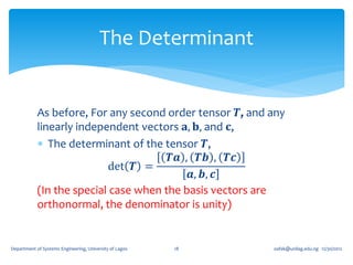
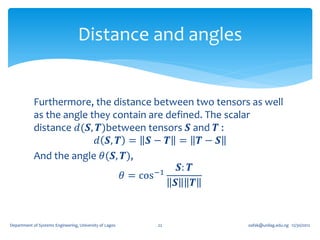
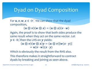
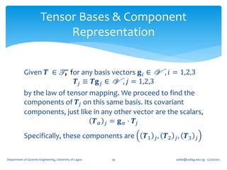
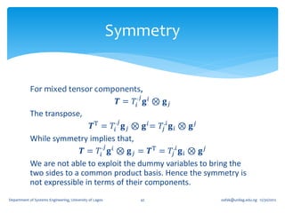
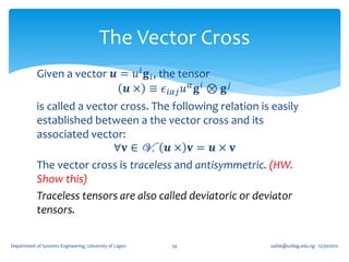
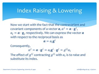
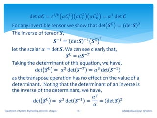
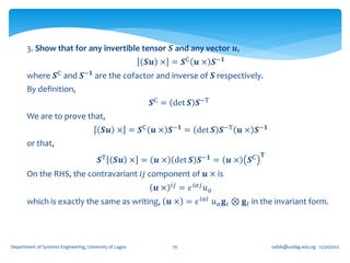
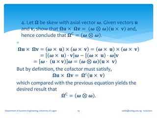
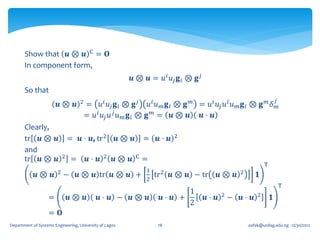
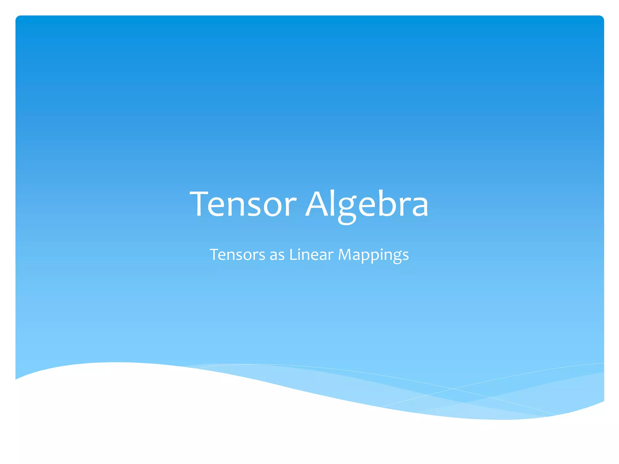
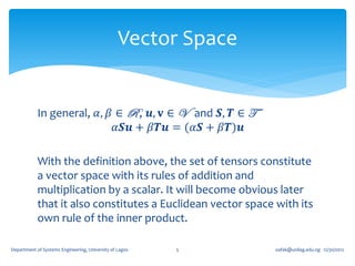
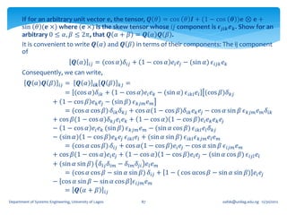
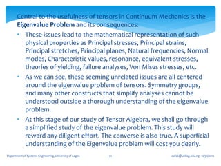
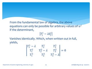
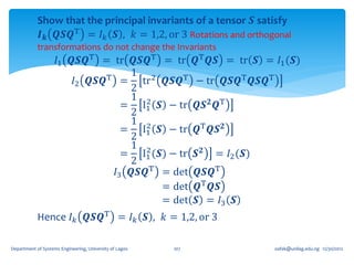
If for an arbitrary unit vector 𝐞, the tensor, 𝑸 𝜃 = cos 𝜃 𝑰 + (1 − cos 𝜽 )𝐞 ⊗
𝐞 + sin 𝜃 (𝐞 ×) where (𝐞 ×) is the skew tensor whose 𝑖𝑗 component is 𝝐 𝒋𝒊𝒌 𝒆 𝒌 ,
show that 𝑸 𝜃 (𝑰 − 𝐞 ⊗ 𝐞) = cos 𝜃 (𝑰 − 𝐞 ⊗ 𝐞) + sin 𝜃 (𝐞 ×).
𝑸 𝜃 𝐞 ⊗ 𝐞 = cos 𝜃 𝐞 ⊗ 𝐞 + (1 − cos 𝜽 )𝐞 ⊗ 𝐞 + sin 𝜃 [𝐞 × 𝐞 ⊗ 𝐞 ]
The last term vanishes immediately on account of the fact that 𝐞 ⊗ 𝐞 is a
symmetric tensor. We therefore have,
𝑸 𝜃 𝐞 ⊗ 𝐞 = cos 𝜃 𝐞 ⊗ 𝐞 + (1 − cos 𝜽 )𝐞 ⊗ 𝐞 = 𝐞 ⊗ 𝐞
which again mean that 𝑸 𝜃 so that
𝑸 𝜃 𝑰 − 𝐞 ⊗ 𝐞 = cos 𝜃 𝑰 + 1 − cos 𝜽 𝐞 ⊗ 𝐞 + sin 𝜃 𝐞× − 𝐞⊗ 𝐞
= 𝑐os 𝜃 𝑰 − 𝐞 ⊗ 𝐞 + sin 𝜃 𝐞 ×
as required.


If for an arbitrary unit vector 𝐞, the tensor, 𝑸 𝜃 = cos 𝜃 𝑰 + (1 − cos 𝜽 )𝐞 ⊗
𝐞 + sin 𝜃 (𝐞 ×) where (𝐞 ×) is the skew tensor whose 𝑖𝑗 component is 𝜖 𝑗𝑖𝑘 𝑒 𝑘 .
Show for an arbitrary vector 𝐮 that 𝐯 = 𝑸 𝜃 𝐮 has the same magnitude as 𝐮.
Given an arbitrary vector 𝐮, compute the vector 𝐯 = 𝑸 𝜃 𝐮. Clearly,
𝐯 = cos 𝜃 𝐮 + 1 − cos 𝜽 𝐮 ⋅ 𝐞 𝐞 + sin 𝜃 𝐞 × 𝐮
The square of the magnitude of 𝐯 is
𝐯⋅ 𝐯= 𝐯 𝟐
= cos 2 𝜃 𝐮 ⋅ 𝐮 + 1 − cos 𝜽 𝟐 𝐮 ⋅ 𝐮 𝟐 + sin2 𝜃 𝐞 × 𝐮 2
+ 2 cos 𝜽 1 − cos 𝜽 𝐮⋅ 𝐞 𝟐
= cos2 𝜃 𝐮 ⋅ 𝐮 + 1 − cos 𝜽 𝐮 ⋅ 𝐞 𝟐 1 − cos 𝜽 + 𝟐 cos 𝜽
+ sin2 𝜃 𝐞 × 𝐮 2
= cos 2 𝜃 𝐮 ⋅ 𝐮 + 1 − cos 𝜽 𝐮 ⋅ 𝐞 𝟐 1 + cos 𝜽 + sin2 𝜃 𝐞 × 𝐮 2

= cos2 𝜃 𝐮 ⋅ 𝐮 + 1 − cos 2 𝜽 𝐮 ⋅ 𝐞 𝟐 + sin2 𝜃 𝐞 × 𝐮 2
= cos2 𝜃 𝐮 ⋅ 𝐮 + sin2 𝜃 𝐮⋅ 𝐞 𝟐+ 𝐞× 𝐮 2
= cos2 𝜃 𝐮 ⋅ 𝐮 + sin2 𝜃 𝐮 ⋅ 𝐮 = 𝐮 ⋅ 𝐮.
The operation of the tensor 𝑸 𝜃 on 𝐮 is independent of 𝜃 and does not change the
magnitude. Furthermore, it is also easy to show that the projection 𝐮 ⋅ 𝐞 of an
arbitrary vector on 𝐞 as well as that of its image 𝐯 ⋅ 𝐞 are the same. The axis of
rotation is therefore in the direction of 𝐞.


If for an arbitrary unit vector 𝐞, the tensor, 𝑸 𝜃 = cos 𝜃 𝑰 + (1 − cos 𝜽 )𝐞 ⊗ 𝐞 +
sin 𝜃 (𝐞 ×) where (𝐞 ×) is the skew tensor whose 𝑖𝑗 component is 𝝐 𝒋𝒊𝒌 𝒆 𝒌 . Show for an
arbitrary 0 ≤ 𝛼, 𝛽 ≤ 2𝜋, that 𝑸 𝛼 + 𝛽 = 𝑸 𝛼 𝑸 𝛽 .
It is convenient to write 𝑸 𝛼 and 𝑸 𝛽 in terms of their components: The ij component
of
𝑸 𝛼 𝑖𝑗 = (cos 𝛼)𝛿 𝑖𝑗 + 1 − cos 𝛼 𝑒 𝑖 𝑒 𝑗 − (sin 𝛼) 𝜖 𝑖𝑗𝑘 𝑒 𝑘
Consequently, we can write,
𝑸 𝛼 𝑸 𝛽 = 𝑸 𝛼 𝒊𝒌 𝑸 𝛽 𝑘𝑗 =
𝑖𝑗
= (cos 𝛼)𝛿 𝑖𝑘 + 1 − cos 𝛼 𝑒 𝑖 𝑒 𝑘 − (sin 𝛼) 𝜖 𝑖𝑘𝑙 𝑒 𝑙 (cos 𝛽)𝛿 𝑘𝑗
+ 1 − cos 𝛽 𝑒 𝑘 𝑒 𝑗 − (sin 𝛽) 𝜖 𝑘𝑗𝑚 𝑒 𝑚
= (cos 𝛼 cos 𝛽) 𝛿 𝑖𝑘 𝛿 𝑘𝑗 + cos 𝛼(1 − cos 𝛽)𝛿 𝑖𝑘 𝑒 𝑘 𝑒 𝑗 − cos 𝛼 sin 𝛽 𝜖 𝑘𝑗𝑚 𝑒 𝑚 𝛿 𝑖𝑘
+ cos 𝛽(1 − cos 𝛼)𝛿 𝑘𝑗 𝑒 𝑖 𝑒 𝑘 + 1 − cos 𝛼 1 − cos 𝛽 𝑒 𝑖 𝑒 𝑘 𝑒 𝑘 𝑒 𝑗
− 1 − cos 𝛼 𝑒 𝑖 𝑒 𝑘 (sin 𝛽) 𝜖 𝑘𝑗𝑚 𝑒 𝑚 − (sin 𝛼 cos 𝛽) 𝜖 𝑖𝑘𝑙 𝑒 𝑙 𝛿 𝑘𝑗
− (sin 𝛼) 1 − cos 𝛽 𝑒 𝑘 𝑒 𝑗 𝜖 𝑖𝑘𝑙 𝑒 𝑙 + (sin 𝛼 sin 𝛽) 𝜖 𝑖𝑘𝑙 𝜖 𝑘𝑗𝑚 𝑒 𝑙 𝑒 𝑚
= (cos 𝛼 cos 𝛽) 𝛿 𝑖𝑗 + cos 𝛼(1 − cos 𝛽)𝑒 𝑖 𝑒 𝑗 − cos 𝛼 sin 𝛽 𝜖 𝑖𝑗𝑚 𝑒 𝑚
+ cos 𝛽(1 − cos 𝛼)𝑒 𝑖 𝑒 𝑗 + 1 − cos 𝛼 1 − cos 𝛽 𝑒 𝑖 𝑒 𝑗 − (sin 𝛼 cos 𝛽) 𝜖 𝑖𝑗𝑙 𝑒 𝑙
+ (sin 𝛼 sin 𝛽) 𝛿 𝑙𝑗 𝛿 𝑖𝑚 − 𝛿 𝑙𝑚 𝛿 𝑗𝑖 𝑒 𝑙 𝑒 𝑚
= (cos 𝛼 cos 𝛽 − sin 𝛼 sin 𝛽) 𝛿 𝑖𝑗 + 1 − ( cos αcos 𝛽 − sin 𝛼 sin 𝛽) 𝑒 𝑖 𝑒 𝑗
− cos 𝛼 sin 𝛽 − sin 𝛼 cos 𝛽 𝜖 𝑖𝑗𝑚 𝑒 𝑚
= 𝑸 𝛼 + 𝛽 𝑖𝑗

Use the results of 52 and 55 above to show that the tensor 𝑸 𝜃 = cos 𝜃 𝑰 + (1 −
cos 𝜽 )𝐞 ⊗ 𝐞 + sin 𝜃 (𝐞 ×) is periodic with a period of 2𝜋.
From 55 we can write that 𝑸 𝛼 + 2𝜋 = 𝑸 𝛼 𝑸 2𝜋 . But from 52, 𝑸 0 =
𝑸 2𝜋 = 𝑰. We therefore have that,
𝑸 𝛼 + 2𝜋 = 𝑸 𝛼 𝑸 2𝜋 = 𝑸 𝛼
which completes the proof. The above results show that 𝑸 𝛼 is a rotation along
the unit vector 𝐞 through an angle 𝛼.


Define Lin+as the set of all tensors with a positive determinant. Show that Lin+ is
invariant under G where is the proper orthogonal group of all rotations, in the
sense that for any tensor 𝐀 ∈ Lin+ 𝐐 ∈ G ⇒ 𝐐𝐀𝐐T ∈ Lin+ .(G285)
Since we are given that 𝐀 ∈ Lin+ , the determinant of 𝐀 is positive. Consider
det 𝐐𝐀𝐐T . We observe the fact that the determinant of a product of tensors is
the product of their determinants (proved above). We see clearly that,
det 𝐐𝐀𝐐T = det 𝐐 × det 𝐀 × det 𝐐T . Since 𝐐 is a rotation, det 𝐐 =
det 𝐐T = 1. Consequently we see that,
det 𝐐𝐀𝐐T = det 𝐐 × det 𝐀 × det 𝐐T
= det 𝐐𝐀𝐐T
= 1 × det 𝐀 × 1
= det 𝐀
Hence the determinant of 𝐐𝐀𝐐T is also positive and therefore 𝐐𝐀𝐐T ∈ Lin+ .


Define Sym as the set of all symmetric tensors. Show that Sym is invariant under G
where is the proper orthogonal group of all rotations, in the sense that for any
tensor A ∈ Sym every 𝐐 ∈ 𝐺 ⇒ 𝐐𝐀𝐐T ∈ Sym. (G285)
Since we are given that A ∈ Sym, we inspect the tensor 𝐐𝐀𝐐T . Its transpose is,
T T
𝐐𝐀𝐐T = 𝐐T 𝐀𝐐T = 𝐐𝐀𝐐T . So that 𝐐𝐀𝐐T is symmetric and therefore
𝐐𝐀𝐐T ∈ Sym. so that the transformation is invariant.


Central to the usefulness of tensors in Continuum Mechanics is the
Eigenvalue Problem and its consequences.
• These issues lead to the mathematical representation of such
physical properties as Principal stresses, Principal strains,
Principal stretches, Principal planes, Natural frequencies, Normal
modes, Characteristic values, resonance, equivalent stresses,
theories of yielding, failure analyses, Von Mises stresses, etc.
• As we can see, these seeming unrelated issues are all centered
around the eigenvalue problem of tensors. Symmetry groups,
and many other constructs that simplify analyses cannot be
understood outside a thorough understanding of the eigenvalue
problem.
• At this stage of our study of Tensor Algebra, we shall go through
a simplified study of the eigenvalue problem. This study will
reward any diligent effort. The converse is also true. A superficial
understanding of the Eigenvalue problem will cost you dearly.

The Eigenvalue Problem

Recall that a tensor 𝑻 is a linear transformation for
𝒖∈V
𝑻: V → V
states that ∃ 𝒘 ∈ V such that,
𝑻𝒖 ≡ 𝑻 𝒖 = 𝒘
Generally, 𝒖 and its image, 𝒘 are independent vectors
for an arbitrary tensor 𝑻. The eigenvalue problem
considers the special case when there is a linear
dependence between 𝒖 and 𝒘.


Eigenvalue Problem

Here the image 𝒘 = 𝜆𝒖 where 𝜆 ∈ R
𝑻𝒖 = 𝜆𝒖
The vector 𝒖, if it can be found, that satisfies the above
equation, is called an eigenvector while the scalar 𝜆 is its
corresponding eigenvalue.
The eigenvalue problem examines the existence of the
eigenvalue and the corresponding eigenvector as well
as their consequences.


In order to obtain such solutions, it is useful to write out
this equation in its component form:
𝑇𝑗 𝑖 𝑢 𝑗 𝐠 𝑖 = 𝜆𝑢 𝑖 𝐠 𝑖
so that,
𝑇𝑗 𝑖 − 𝜆𝛿 𝑗𝑖 𝑢 𝑗 𝐠 𝑖 = 𝐨
the zero vector. Each component must vanish
identically so that we can write
𝑇𝑗 𝑖 − 𝜆𝛿 𝑗𝑖 𝑢 𝑗 = 0


From the fundamental law of algebra, the above
equations can only be possible for arbitrary values of 𝑢 𝑗
if the determinant,
𝑇𝑗 𝑖 − 𝜆𝛿 𝑗𝑖
Vanishes identically. Which, when written out in full,
yields,
1 1 1
𝑇1 − 𝜆 𝑇2 𝑇3
2 2 2 =0
𝑇1 𝑇2 − 𝜆 𝑇3
3 3 3
𝑇1 𝑇2 𝑇3 − 𝜆


Expanding, we have,
1 2 3 1 2 3 1 2 3 1 2 3 1 2 3
−𝑇3 𝑇2 𝑇1 + 𝑇2 𝑇3 𝑇1 + 𝑇3 𝑇1 𝑇2 − 𝑇1 𝑇3 𝑇2 − 𝑇2 𝑇1 𝑇3
1 2 3 1 2 1 2 1 3 2 3
+ 𝑇1 𝑇2 𝑇3 + 𝑇2 𝑇1 𝜆 − 𝑇1 𝑇2 𝜆 + 𝑇3 𝑇1 𝜆 + 𝑇3 𝑇2 𝜆
1 3 2 3 1 2 3
− 𝑇1 𝑇3 𝜆 − 𝑇2 𝑇3 𝜆 + 𝑇1 𝜆2 + 𝑇2 𝜆2 + 𝑇3 𝜆2 − 𝜆3
=0
1 2 3 1 2 3 1 2 3 1 2 3 1 2 3
= −𝑇3 𝑇2 𝑇1 + 𝑇2 𝑇3 𝑇1 + 𝑇3 𝑇1 𝑇2 − 𝑇1 𝑇3 𝑇2 − 𝑇2 𝑇1 𝑇3
1 2 3
+ 𝑇1 𝑇2 𝑇3
1 2 1 2 1 3 2 3 1 3
+ ( 𝑇2 𝑇1 − 𝑇1 𝑇2 + 𝑇3 𝑇1 + 𝑇3 𝑇2 − 𝑇1 𝑇3
2 3 1 2 3
− 𝑇2 𝑇3 ) 𝜆 + 𝑇1 + 𝑇2 + 𝑇3 𝜆2 − 𝜆3 = 0
or
𝜆3 − 𝐼1 𝜆2 + 𝐼2 𝜆 − 𝐼3 = 0


Principal Invariants Again

 This is the characteristic equation for the tensor 𝑻.
From here we are able, in the best cases, to find the
three eigenvalues. Each of these can be used in to
obtain the corresponding eigenvector.
 The above coefficients are the same invariants we
have seen earlier!


Positive Definite Tensors

A tensor 𝑻 is Positive Definite if for all 𝒖 ∈ V ,
𝒖 ⋅ 𝑻𝒖 > 0
It is easy to show that the eigenvalues of a symmetric,
positive definite tensor are all greater than zero. (HW:
Show this, and its converse that if the eigenvalues are
greater than zero, the tensor is symmetric and positive
definite. Hint, use the spectral decomposition.)


Cayley- Hamilton Theorem

 We now state without proof (See Dill for proof) the
important Caley-Hamilton theorem: Every tensor
satisfies its own characteristic equation. That is, the
characteristic equation not only applies to the
eigenvalues but must be satisfied by the tensor 𝐓
itself. This means,
𝐓 3 − 𝐼1 𝐓 2 + 𝐼2 𝐓 − 𝐼3 𝟏 = 𝑶
is also valid.
 This fact is used in continuum mechanics to obtain the
spectral decomposition of important material and
spatial tensors.


Spectral Decomposition
 It is easy to show that when the tensor is symmetric, its
three eigenvalues are all real. When they are distinct,
corresponding eigenvectors are orthogonal. It is
therefore possible to create a basis for the tensor with an
orthonormal system based on the normalized
eigenvectors. This leads to what is called a spectral
decomposition of a symmetric tensor in terms of a
coordinate system formed by its eigenvectors:
3

𝐓= 𝜆 𝑖 𝐧 𝑖 ⨂𝐧 𝑖
𝑖=1
Where 𝐧 𝑖 is the normalized eigenvector corresponding to
the eigenvalue 𝜆 𝑖 .

Multiplicity of Roots

 The above spectral decomposition is a special case
where the eigenbasis forms an Orthonormal Basis.
Clearly, all symmetric tensors are diagonalizable.
 Multiplicity of roots, when it occurs robs this
representation of its uniqueness because two or
more coefficients of the eigenbasis are now the same.
 The uniqueness is recoverable by the ingenious
device of eigenprojection.


Eigenprojectors

Case 1: All Roots equal.
 The three orthonormal eigenvectors in an ONB
obviously constitutes an Identity tensor 𝟏. The unique
spectral representation therefore becomes
3 3

𝐓= 𝜆 𝑖 𝐧 𝑖 ⨂𝐧 𝑖 = 𝜆 𝐧 𝑖 ⨂𝐧 𝑖
𝑖=1 𝑖=1
since 𝜆1 = 𝜆2 = 𝜆3 = 𝜆 in this case.


Eigenprojectors

Case 2: Two Roots equal: 𝜆1 unique while 𝜆2 = 𝜆3
In this case,
𝐓 = 𝜆1 𝐧1 ⨂𝐧1 + 𝜆2 𝟏 − 𝐧1 ⨂𝐧1
since 𝜆2 = 𝜆3 in this case.
The eigenspace of the tensor is made up of the projectors:
𝑷1 = 𝐧1 ⨂𝐧1
and
𝑷2 = 𝟏 − 𝐧2 ⨂𝐧2


Eigenprojectors

The eigen projectors in all cases are based on the
normalized eigenvectors of the tensor. They constitute
the eigenspace even in the case of repeated roots. They
can be easily shown to be:
1. Idempotent: 𝑷 𝑖 𝑷 𝑖 = 𝑷 𝑖 (no sums)
2. Orthogonal: 𝑷 𝑖 𝑷 𝑗 = 𝑶 (the anihilator)
𝑛
3. Complete: 𝑖=1 𝑷 𝑖 = 𝟏 (the identity)


Tensor Functions
 For symmetric tensors (with real eigenvalues and
consequently, a defined spectral form in all cases),
the tensor equivalent of real functions can easily be
defined:
 Trancendental as well as other functions of tensors
are defined by the following maps:
𝑭: Sym → Sym
Maps a symmetric tensor into a symmetric tensor. The
latter is the spectral form such that,
3

𝑭 𝑻 ≡ 𝑓(𝜆 𝑖 )𝐧 𝑖 ⨂𝐧 𝑖
𝑖=1

Tensor functions

 Where 𝑓(𝜆 𝑖 ) is the relevant real function of the ith
eigenvalue of the tensor 𝑻.
 Whenever the tensor is symmetric, for any map,
𝑓:R → R, ∃ 𝑭: Sym → Sym
As defined above. The tensor function is defined
uniquely through its spectral representation.


Show that the principal invariants of a tensor 𝑺 satisfy
𝑰 𝒌 𝑸𝑺𝑸T = 𝐼 𝑘 𝑺 , 𝑘 = 1,2, or 3 Rotations and orthogonal
transformations do not change the Invariants
𝐼1 𝑸𝑺𝑸T = tr 𝑸𝑺𝑸T = tr 𝑸T 𝑸𝑺 = tr 𝑺 = 𝐼1 (𝑺)
T =
1 2
𝐼2 𝑸𝑺𝑸 tr 𝑸𝑺𝑸T − tr 𝑸𝑺𝑸T 𝑸𝑺𝑸T
2
1 2
= I1 𝑺 − tr 𝑸𝑺 𝟐 𝑸T
2
1 2
= I1 𝑺 − tr 𝑸T 𝑸𝑺 𝟐
2
1 2
= I1 (𝑺) − tr 𝑺𝟐 = 𝐼2 (𝑺)
2
𝐼3 𝑸𝑺𝑸T = det 𝑸𝑺𝑸T
= det 𝑸T 𝑸𝑺
= det 𝑺 = 𝐼3 𝑺
Hence 𝐼 𝑘 𝑸𝑺𝑸T = 𝐼 𝑘 𝑺 , 𝑘 = 1,2, or 3


2
Show that, for any tensor 𝑺, tr 𝑺2 = 𝐼1 (𝑺) − 2𝐼2 𝑺 and
3
tr 𝑺3 = 𝐼1 𝑺 − 3𝐼1 𝐼2 𝑺 + 3𝐼3 𝑺

1 2
𝐼2 𝑺 = tr 𝑺 − tr 𝑺2
2
1 2
= 𝐼1 (𝑺) − tr 𝑺2
2
So that,
2
tr 𝑺2 = 𝐼1 (𝑺) − 2𝐼2 𝑺
By the Cayley-Hamilton theorem,
𝑺3 − 𝐼1 𝑺2 + 𝐼2 𝑺 − 𝐼3 𝟏 = 𝟎
Taking a trace of the above equation, we can write that,
tr 𝑺3 − 𝐼1 𝑺2 + 𝐼2 𝑺 − 𝐼3 𝟏 = tr(𝑺3 ) − 𝐼1 tr 𝑺2 + 𝐼2 tr 𝑺 − 3𝐼3 = 0
so that,
tr 𝑺3 = 𝐼1 𝑺 tr 𝑺2 − 𝐼2 𝑺 tr 𝑺 + 3𝐼3 𝑺
2
= 𝐼1 𝑺 𝐼1 𝑺 − 2𝐼2 𝑺 − 𝐼1 𝑺 𝐼2 𝑺 + 3𝐼3 𝑺
3
= 𝐼1 𝑺 − 3𝐼1 𝐼2 𝑺 + 3𝐼3 𝑺
As required.

Suppose that 𝑼 and 𝑪 are symmetric, positive-definite
tensors with 𝑼2 = 𝑪, write the invariants of C in terms
of U
2
𝐼1 𝑪 = tr 𝑼2 = 𝐼1 (𝑼) − 2𝐼2 𝑼
By the Cayley-Hamilton theorem,
𝑼3 − 𝐼1 𝑼2 + 𝐼2 𝑼 − 𝐼3 𝑰 = 𝟎
which contracted with 𝑼 gives,
𝑼4 − 𝐼1 𝑼3 + 𝐼2 𝑼2 − 𝐼3 𝑼 = 𝟎
so that,
𝑼4 = 𝐼1 𝑼3 − 𝐼2 𝑼2 + 𝐼3 𝑼
and
tr 𝑼4 = 𝐼1 tr 𝑼3 − 𝐼2 tr 𝑼2 + 𝐼3 tr 𝑼
3
= 𝐼1 𝑼 𝐼1 𝑼 − 3𝐼1 𝑼 𝐼2 𝑼 + 3𝐼3 𝑼
2
− 𝐼2 𝑼 𝐼1 𝑼 − 2𝐼2 𝑼 + 𝐼1 𝑼 𝐼3 𝑼
4 2 2
= 𝐼1 𝑼 − 4𝐼1 𝑼 𝐼2 𝑼 + 4𝐼1 𝑼 𝐼3 𝑼 + 2𝐼2 𝑼

But,
1 2 2
1 2 2
𝐼2 𝑪 = 𝐼1 𝑪 − tr 𝑪 = 𝐼1 𝑼 − tr 𝑼4
2 2
1 2 2
= tr 𝑼 − tr 𝑼4
2
1 2 2
= 𝐼1 𝑼 − 2𝐼2 𝑼 − tr 𝑼4
2
1 4 2 2
= 𝐼1 𝑼 − 4𝐼1 𝑼 𝐼2 𝑼 + 4𝐼2 𝑼
2
4 2 2
− 𝐼1 𝑼 − 4𝐼1 𝑼 𝐼2 𝑼 + 4𝐼1 𝑼 𝐼3 𝑼 + 2𝐼2 𝑼
The boxed items cancel out so that,
2
𝐼2 𝑪 = 𝐼2 𝑼 − 2𝐼1 𝑼 𝐼3 𝑼
as required.
2
𝐼3 𝑪 = det 𝑪 = det 𝑼2 = det 𝑼 2 = 𝐼3 𝑼


2. tensor algebra jan 2013

More Related Content

What's hot

Viewers also liked

Similar to 2. tensor algebra jan 2013

Recently uploaded

2. tensor algebra jan 2013