Download to read offline


![24
A.2 Tensors
A.2.1 Definitions
A tensor (2nd order) has nine components, for example, a stress tensor
can be expressed in rectangular coordinates listed in the following:
A.2.2 Product
The tensor product of two vectors v and w, denoted as vw, is a tensor defined by
xx xy xz
yx yy yz
zx zy zz
τ
x x x x y x z
y x y z y x y y y z
z x z y z z
z
v v w v w v w
v w w w v w v w v w
v w v w v w
v
vw
[A.2-1]
[A.2-2]
Explanation (Borisenko, p64)](https://image.slidesharecdn.com/vectorandtensor-230101164403-3b04799e/75/vector-and-tensor-pptx-24-2048.jpg)
![25
The vector product of a tensor and a vector v, denoted by .v is a vector defined by
x
xx xy xz
yx yy yz y
zx zy zz z
x xx y xy z xz x yx y yy z yz
x zx y zy z zz
x y
z
v
v v
v
v v v v v v
v v v
τ
e e
e
[A.2-3]
x
x x x y x z
y x y y y z y
z x z y z z z
x x x x y y x z z y x x y y y y z z
z x x z y y z z z
x y z x x y y z z
x y
z
x y z
n
v v v v v v
v v v v v v n
v v v v v v n
v v n v v n v v n v v n v v n v v n
v v n v v n v v n
v v v v n v n v n
vv n
e e
e
e e e
v v n [A.2-5]
The product between a tensor vv and a vector n is a vector](https://image.slidesharecdn.com/vectorandtensor-230101164403-3b04799e/75/vector-and-tensor-pptx-25-2048.jpg)
![26
The scalar product of two tensors s and , denoted as s:, is a scalar defined by
: :
xx xy xz xx xy xz
yx yy yz yx yy yz
zx zy zz zx zy zz
xx xx xy yx xz zx yx xy yy yy yz zy
zx xz zy yz zz zz
s s s
s s s
s s s
s s s s s s
s s s
σ τ
[A.2-6]
: :
x x x y x z xx xy xz
y x y y y z yx yy yz
z x z y z z zx zy zz
x x xx x y yx x z zx y x xy y y yy y z zy
z x xz z y yz z z zz
v w v w v w
v w v w v w
v w v w v w
v w v w v w v w v w v w
v w v w v w
vw [A.2-7]
The scalar product of two tensors vw and is
Physical quantity Multiplication sign
Scalar Vector Tensor None X ‧ :
Order 0 1 2 0 -1 -2 -4
Table A.1-1 Orders of physical quantities and their multiplication signs](https://image.slidesharecdn.com/vectorandtensor-230101164403-3b04799e/75/vector-and-tensor-pptx-26-2048.jpg)
![2
x y z
x y z
e e e
x y z
s s s
s
x y z
e e e
A.3 Differential Operators
A.3.1 Definitions
The vector differential operation , called “del”, has components similar to those
of a vector. However, unlike a vector, it cannot stand alone and must operate on
a scalar, vector, or tensor function. In rectangular coordinates it is defined by
The gradient of a scalar field s, denoted as ▽ s, is a vector defined by
[A.3-1]
[A.3-2]
A.3.2 Products
The divergence of a vector field v, denoted as ▽‧v is a scalar .
[A.3-5]
v x y z x x y y z z
x y z
v v v
x y z
v v v
x y z
e e e e e e
Flux is defined as the amount that flows through a unit area per unit time
Flow rate is the volume of fluid which passes through a given surface per unit time](https://image.slidesharecdn.com/vectorandtensor-230101164403-3b04799e/75/vector-and-tensor-pptx-27-2048.jpg)
![28
x y z x x y y z z
x y z
x y z
x y z
a av av av
x y z
av av av
x y z
v v v a a a
a v v v
x y z x y z
v e e e e e e
Similarly
[A.3-5]
For the operation of [A.3-7]
a a a
v v v
For the operation of ▽‧▽s, we have
[A.3-8]
[A.3-9]
2
2
2
2
2
2
)
e
e
e
(
)
e
e
e
(
z
s
y
s
x
s
z
s
y
s
x
s
z
y
x
s z
y
x
z
y
x
In other words s
s 2
Where the differential operator▽2, called Laplace operator, is defined as
2
2
2
2
2
2
2
z
y
x
[A.3-10]
For example: Streamline is defined as a line everywhere tangent to the velocity
vector at a given instant and can be described as a scale function of f.
Lines of constant f are streamlines of the flow for inviscid irrotational flow
in the xy plane ▽2f=0](https://image.slidesharecdn.com/vectorandtensor-230101164403-3b04799e/75/vector-and-tensor-pptx-28-2048.jpg)
![29
x y z
x y z
e e e
x y z
v v v
v
x y z
x y z
x y z
x y z
v v v
x x x x
v v v
v v v
y y y y
v v v
z z z z
v
The curl of a vector field v, denoted by ▽ x v, is a vector like the vector product
of two vectors.
[A.3-11]
[A.3-12]
Like the tensor product of two vectors, ▽v is a tensor as shown:
x y x z y x
x y z
v v v v v v
e e e
y z z x x y
When the flow is irrotational, v = 0
](https://image.slidesharecdn.com/vectorandtensor-230101164403-3b04799e/75/vector-and-tensor-pptx-29-2048.jpg)
![30
[A.3-13]
Like the vector product of a vector and a tensor, ▽‧ is a vector.
xx xy xz
yx yy yz
zx zy zz
yx xy yy zy
xx zx
yz
xz zz
x y
z
x y z
x y z x y z
x y z
τ
e e
e
x x x y x z
y x y y y z
z x z y z z
x x x y x z x
y x y y y z y
z x z y z z z
v v v v v v
v v v v v v
x y z
v v v v v v
v v v v v v
x y z
v v v v v v
x y z
v v v v v v
x y z
vv
e
e
e
[A.3-14]
From Eq. [A.2-2]
[A.3-15]
It can be shown that
vv v v v v](https://image.slidesharecdn.com/vectorandtensor-230101164403-3b04799e/75/vector-and-tensor-pptx-30-2048.jpg)


![73
A.4 Divergence Theorem
A.4.1 Vectors
Let Ω be a closed region in space surrounded by a surface A and n the outward-
directed unit vector normal to the surface. For a vector v
A
d dA
v v n [A.4-1]
This equation , called the gauss divergence theorem, is useful for converting from a
surface integral to a volume integral.
A.4.2 Scalars
A.4.3 Tensors
For a scale s
For a tensor or vv
A
sd s dA
n
A
d dA
n
A
d dA
vv vv n
[A.4-2]
[A.4-3]
[A.4-4]](https://image.slidesharecdn.com/vectorandtensor-230101164403-3b04799e/75/vector-and-tensor-pptx-73-2048.jpg)


![88
Fig. A.5-1(b)
A.5.1 Cylindrical Coordinates
For cylindrical coordinates, as shown in A.5-1(b), the variables r, θ, and z are
related to x, y, and z.
x = r cosθ [A.5-1] y = r sinθ [A.5-2] z = z [A.5-3]
Fig. A.5-1(b)*
v = er vr + eθvθ + ezvz
rr r rz
r z
zr z zz
τ
and
The differential increments of a control unit, as shown in Fig. A.5-1(b)*, in r, ,
and z axis are dr, rd , and dz, respectively. A vector v and a tensor τcan be
expressed as follows:](https://image.slidesharecdn.com/vectorandtensor-230101164403-3b04799e/75/vector-and-tensor-pptx-88-2048.jpg)
![89
Fig. A.5-1(c)
A.5.2 Spherical Coordinates
For spherical coordinates, as shown in A.5-1(c), the variables r, θ, and ψ are
related to x, y, and z as follows
x= r sin cosf A.5-6
y = r sin sinf [A.5-7]
z = r cos A.5-8
[A.5-9]
rr r rz
r z
zr z zz
τ [A.5-10]
The differential increments of a control
unit, as shown in Fig. A.5-1(c)*, in r, θ,
and φ axis are dr, rdθ , and rsinθdφ ,
respectively. A vector v and a tensor τ
can be expressed as follows:
f
f
v
v
vr
r e
e
e
v
Fig. A.5-1(c)*
θ
φ φ
θ
θ φ
θ
θ](https://image.slidesharecdn.com/vectorandtensor-230101164403-3b04799e/75/vector-and-tensor-pptx-89-2048.jpg)
![90
A.5.3 Differential Operators
1
0
0
rz
r z
zr z zz
r zr
rr r
r
r rr z
τ e
e e e
1
0
0
r
r
r
r r
rr r
r
r rr
τ e
e e e
1
r z
s s s
s
r r z
e e e
1 1
sin
r
s s s
s
r r r
f
f
e e e
Vectors, tensors, and their products in curvilinear coordinates are similar in form
to those in curvilinear coordinates. For example, if v = er in cylindrical coordinates,
the operation of τ.er can be expressed in [A.5-11], and it can be expressed in
[A.5-12] when in spherical coordinates
[A.5-11] [A.5-12]
In curvilinear coordinates, ▽ assumes different forms depending on the orders of
the physical quantities and the multiplication sign involved. For example, in cylindrical
coordinates
Whereas in spherical coordinates,
[A.5-13]
[A.5-14]](https://image.slidesharecdn.com/vectorandtensor-230101164403-3b04799e/75/vector-and-tensor-pptx-90-2048.jpg)


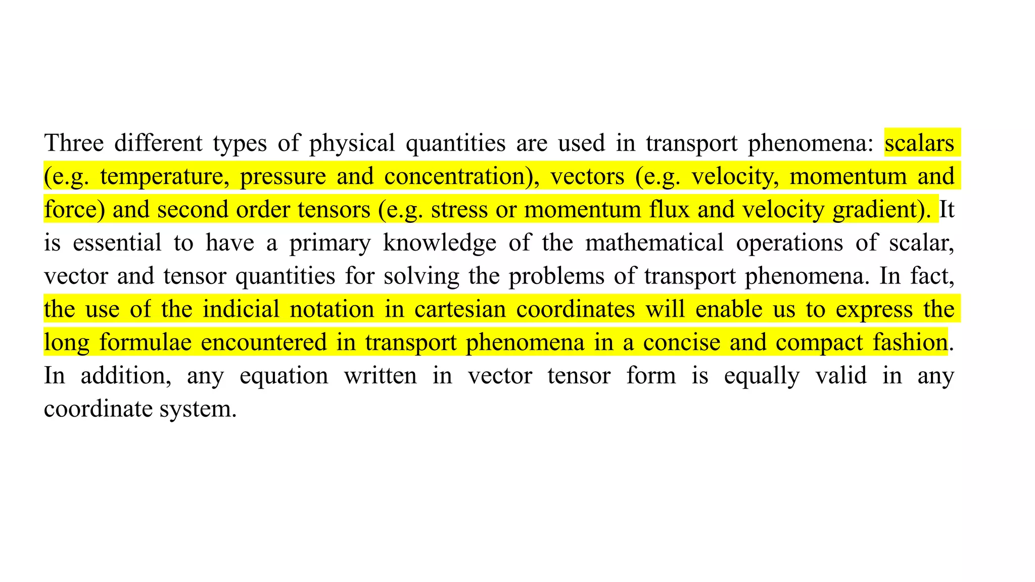
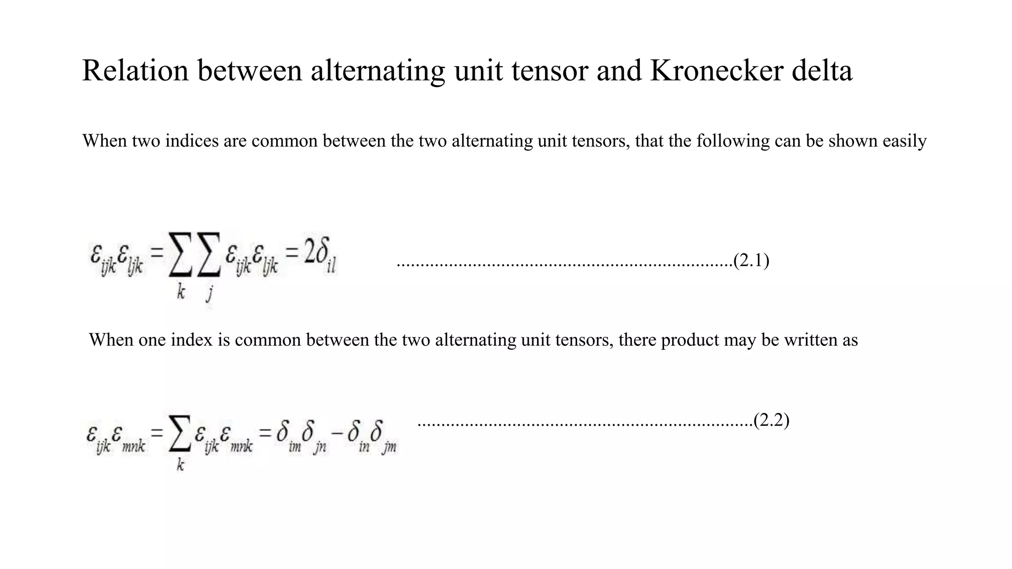
This document provides an introduction to transport phenomena and the key concepts involved. It discusses the three main types of transport - momentum, heat, and mass. Vector and tensor analysis concepts are also introduced, which are essential for solving transport phenomena problems. These include scalar, vector, and tensor quantities, and differential operators like gradient and divergence. Key topics in vector and tensor analysis like Kronecker delta, alternating unit tensor, and index notation are also covered at a high level.