Downloaded 20,604 times


![2-18
When the above two expressions for A/8B and A are substituted into the above expression for E0 (- 5.37 eV), the
following results
−5.37 eV = = − A
A
8B
⎛
⎜
⎝
−1/7 + B
⎞
⎟
⎠
A
10B
⎛
⎜
⎝
−8/7
⎞
⎟
⎠
= − 8B(0.38 nm)-7
[(0.38 nm)-7]−1/7 + B
[(0.38 nm)-7]−8/7
= − 8B(0.38 nm)-7
0.38 nm
+ B
(0.38 nm)8
Or
−5.37 eV = = − 8B
(0.38 nm)8 + B
(0.38 nm)8 = − 7B
(0.38 nm)8
Solving for B from this equation yields
B = 3.34 × 10⁻⁴ eV- nm8
Furthermore, the value of A is determined from one of the previous equations, as follows:
A = 8B(0.38 nm)-7 = (8)(3.34 × 10⁻⁴ eV - nm8 )(0.38 nm)-7
= 2.34 eV- nm
Thus, Equations 2.8 and 2.9 become
EA = − 2.34
r
ER = 3.34 x 10⁻⁴
r8
Of course these expressions are valid for r and E in units of nanometers and electron volts, respectively.
Excerpts from this work may be reproduced by instructors for distribution on a not-for-profit basis for testing or instructional purposes only to
students enrolled in courses for which the textbook has been adopted. Any other reproduction or translation of this work beyond that permitted
by Sections 107 or 108 of the 1976 United States Copyright Act without the permission of the copyright owner is unlawful.](https://image.slidesharecdn.com/ecyluo1ys2qvoutji72q-signature-9b381c5777758ee4fe884904ded9f35d0b251da572c8ac51c821cb24bd095f1b-poli-141018125101-conversion-gate02/85/solution-for-Materials-Science-and-Engineering-7th-edition-by-William-D-Callister-Jr-18-320.jpg)


![3-8
Density Computations
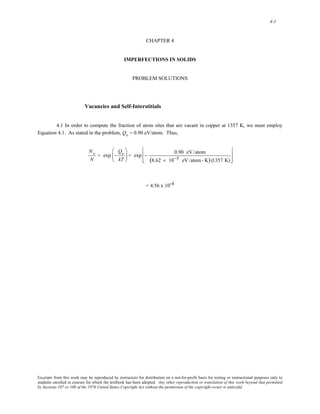
3.7 This problem calls for a computation of the density of molybdenum. According to Equation 3.5
ρ =
nAMo
VCNA
For BCC, n = 2 atoms/unit cell, and
VC = 4R
3
⎛
⎜
⎝
⎞
⎟
⎠
3
Thus,
ρ =
nAMo
4 R
3
⎛
⎜
⎝
⎞
⎟
⎠
3
NA
= (2 atoms/unit cell)(95.94 g/mol)
[(4) (0.1363 × 10⁻⁷ cm)3 / 3]3
/(unit cell) (6.023 × 10²³ atoms/mol)
= 10.21 g/cm3
The value given inside the front cover is 10.22 g/cm3.
Excerpts from this work may be reproduced by instructors for distribution on a not-for-profit basis for testing or instructional purposes only to
students enrolled in courses for which the textbook has been adopted. Any other reproduction or translation of this work beyond that permitted
by Sections 107 or 108 of the 1976 United States Copyright Act without the permission of the copyright owner is unlawful.](https://image.slidesharecdn.com/ecyluo1ys2qvoutji72q-signature-9b381c5777758ee4fe884904ded9f35d0b251da572c8ac51c821cb24bd095f1b-poli-141018125101-conversion-gate02/85/solution-for-Materials-Science-and-Engineering-7th-edition-by-William-D-Callister-Jr-33-320.jpg)


![3-13
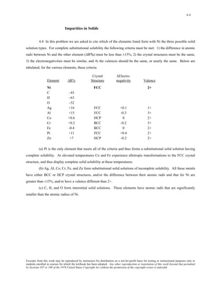
3.12 This problem asks that we calculate the theoretical densities of Al, Ni, Mg, and W.
Since Al has an FCC crystal structure, n = 4, and VC = 1 6R3 2 (Equation 3.4). Also, R = 0.143 nm (1.43
x 10-8 cm) and AAl = 26.98 g/mol. Employment of Equation 3.5 yields
ρ =
nAAl
VC NA
= (4 atoms/unit cell)(26.98 g/mol)
[(2)(1.43 x 10⁻⁸ cm)( 2)]3
/(unit cell)
⎧
⎨
⎩
⎫
⎬
⎭
(6.023 x 10²³ atoms/mol)
= 2.71 g/cm3
The value given in the table inside the front cover is 2.71 g/cm3.
Nickel also has an FCC crystal structure and therefore
ρ = (4 atoms/unit cell)(58.69 g/mol)
[(2)(1.25 x 10⁻⁸ cm)( 2)]3
/(unit cell )
⎧
⎨
⎩
⎫
⎬
⎭
(6.023 x 10²³ atoms/mol)
= 8.82 g/cm3
The value given in the table is 8.90 g/cm3.
Magnesium has an HCP crystal structure, and from the solution to Problem 3.6,
VC = 3 3a2c
2
and, since c = 1.624a and a = 2R = 2(1.60 x 10⁻⁸ cm) = 3.20 x 10⁻⁸ cm
VC = (3 3)(1.624)(3.20 x 10⁻⁸ cm)3
2
= 1.38 x 10⁻²² cm3/unit cell
Also, there are 6 atoms/unit cell for HCP. Therefore the theoretical density is
ρ =
nAMg
VC NA
Excerpts from this work may be reproduced by instructors for distribution on a not-for-profit basis for testing or instructional purposes only to
students enrolled in courses for which the textbook has been adopted. Any other reproduction or translation of this work beyond that permitted
by Sections 107 or 108 of the 1976 United States Copyright Act without the permission of the copyright owner is unlawful.](https://image.slidesharecdn.com/ecyluo1ys2qvoutji72q-signature-9b381c5777758ee4fe884904ded9f35d0b251da572c8ac51c821cb24bd095f1b-poli-141018125101-conversion-gate02/85/solution-for-Materials-Science-and-Engineering-7th-edition-by-William-D-Callister-Jr-38-320.jpg)

![3-15
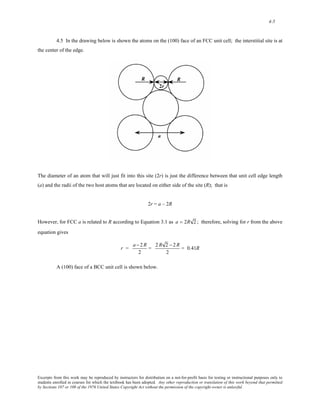
3.13 In order to determine whether Nb has an FCC or a BCC crystal structure, we need to compute its
density for each of the crystal structures. For FCC, n = 4, and a = 2R 2 (Equation 3.1). Also, from Figure 2.6, its
atomic weight is 92.91 g/mol. Thus, for FCC (employing Equation 3.5)
ρ =
nANb
a3NA
=
nANb
(2R 2)3NA
= (4 atoms/unit cell)(92.91 g/mol)
[(2)(1.43 × 10⁻⁸ cm)( 2)]3
/(unit cell)
⎧
⎨
⎩
⎫
⎬
⎭
(6.023 × 10²³ atoms /mol)
= 9.33 g/cm3
For BCC, n = 2, and a =
4R
3
(Equation 3.3), thus
ρ =
nANb
4 R
3
⎛
⎜⎜
⎝
⎞
⎟⎟
⎠
3
NA
ρ = (2 atoms/unit cell)(92.91 g/mol)
(4)(1.43 × 10⁻⁸ cm)
3
⎡
⎢
⎣
⎢
⎤
⎥
⎦
⎥
3
/(unit cell)
⎧
⎨
⎪
⎩⎪
⎫
⎬
⎪
⎪⎭
(6.023 × 10²³ atoms /mol)
= 8.57 g/cm3
which is the value provided in the problem statement. Therefore, Nb has a BCC crystal structure.
Excerpts from this work may be reproduced by instructors for distribution on a not-for-profit basis for testing or instructional purposes only to
students enrolled in courses for which the textbook has been adopted. Any other reproduction or translation of this work beyond that permitted
by Sections 107 or 108 of the 1976 United States Copyright Act without the permission of the copyright owner is unlawful.](https://image.slidesharecdn.com/ecyluo1ys2qvoutji72q-signature-9b381c5777758ee4fe884904ded9f35d0b251da572c8ac51c821cb24bd095f1b-poli-141018125101-conversion-gate02/85/solution-for-Materials-Science-and-Engineering-7th-edition-by-William-D-Callister-Jr-40-320.jpg)
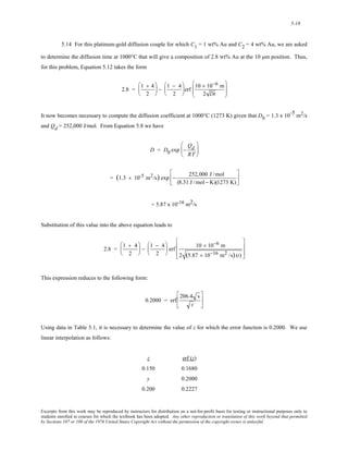
![3-16
3.14 For each of these three alloys we need, by trial and error, to calculate the density using Equation 3.5,
and compare it to the value cited in the problem. For SC, BCC, and FCC crystal structures, the respective values of
n are 1, 2, and 4, whereas the expressions for a (since VC = a3) are 2R, 2 R 2 , and
4R
3
.
For alloy A, let us calculate ρ assuming a BCC crystal structure.
ρ =
nAA
VC NA
=
nAA
4R
3
⎛
⎜
⎝
⎞
⎟
⎠
3
NA
= (2 atoms/unit cell)(43.1 g/mol)
(4)(1.22 × 10⁻⁸ cm)
3
⎡
⎢
⎣
⎢
3
/(unit cell)
⎤
⎥
⎦
⎥
⎧
⎨
⎪
⎩⎪
⎫
⎬
⎪
⎪⎭
(6.023 × 10²³ atoms/mol)
= 6.40 g/cm3
Therefore, its crystal structure is BCC.
For alloy B, let us calculate ρ assuming a simple cubic crystal structure.
ρ =
nAB
(2a)3NA
= (1 atom/unit cell)(184.4 g/mol)
[(2)(1.46 × 10⁻⁸ cm)]3
/(unit cell)
⎧
⎨
⎩
⎫
⎬
⎭
(6.023 × 10²³ atoms/mol)
= 12.3 g/cm3
Therefore, its crystal structure is simple cubic.
For alloy C, let us calculate ρ assuming a BCC crystal structure.
Excerpts from this work may be reproduced by instructors for distribution on a not-for-profit basis for testing or instructional purposes only to
students enrolled in courses for which the textbook has been adopted. Any other reproduction or translation of this work beyond that permitted
by Sections 107 or 108 of the 1976 United States Copyright Act without the permission of the copyright owner is unlawful.](https://image.slidesharecdn.com/ecyluo1ys2qvoutji72q-signature-9b381c5777758ee4fe884904ded9f35d0b251da572c8ac51c821cb24bd095f1b-poli-141018125101-conversion-gate02/85/solution-for-Materials-Science-and-Engineering-7th-edition-by-William-D-Callister-Jr-41-320.jpg)


= 7.31 g/cm3
Excerpts from this work may be reproduced by instructors for distribution on a not-for-profit basis for testing or instructional purposes only to
students enrolled in courses for which the textbook has been adopted. Any other reproduction or translation of this work beyond that permitted
by Sections 107 or 108 of the 1976 United States Copyright Act without the permission of the copyright owner is unlawful.](https://image.slidesharecdn.com/ecyluo1ys2qvoutji72q-signature-9b381c5777758ee4fe884904ded9f35d0b251da572c8ac51c821cb24bd095f1b-poli-141018125101-conversion-gate02/85/solution-for-Materials-Science-and-Engineering-7th-edition-by-William-D-Callister-Jr-44-320.jpg)
![3-20
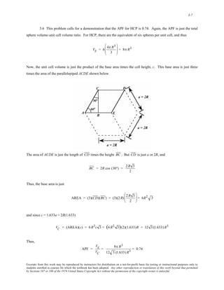
3. 17 (a) We are asked to calculate the unit cell volume for Be. For HCP, from the solution to Problem
3.6
V C = 6R2c 3
But, c = 1.568a, and a = 2R, or c = 3.14R, and
V C = (6)(3.14) R3 3
= (6)(3.14) ( 3) [0.1143 × 10⁻⁷ cm]3
= 4.87 × 10⁻²³ cm3/unit cell
(b) The theoretical density of Be is determined, using Equation 3.5, as follows:
ρ =
nABe
VC NA
For HCP, n = 6 atoms/unit cell, and for Be, ABe = 9.01 g/mol (as noted inside the front cover). Thus,
ρ = (6 atoms/unit cell)(9.01 g/mol)
(4.87 × 10⁻²³ cm3/unit cell)(6.023 × 10²³ atoms/mol)
= 1.84 g/cm3
The value given in the literature is 1.85 g/cm3.
Excerpts from this work may be reproduced by instructors for distribution on a not-for-profit basis for testing or instructional purposes only to
students enrolled in courses for which the textbook has been adopted. Any other reproduction or translation of this work beyond that permitted
by Sections 107 or 108 of the 1976 United States Copyright Act without the permission of the copyright owner is unlawful.](https://image.slidesharecdn.com/ecyluo1ys2qvoutji72q-signature-9b381c5777758ee4fe884904ded9f35d0b251da572c8ac51c821cb24bd095f1b-poli-141018125101-conversion-gate02/85/solution-for-Materials-Science-and-Engineering-7th-edition-by-William-D-Callister-Jr-45-320.jpg)


![3-30
represent any bonds at all (in which case we click on the “Go to Step 4” button). If it is decided to show bonds,
probably the best thing to do is to represent unit cell edges as bonds.
The window in Step 4 presents all the data that have been entered; you may review these data for
accuracy. If any changes are required, it is necessary to close out all windows back to the one in which corrections
are to be made, and then reenter data in succeeding windows. When you are fully satisfied with your data, click on
the “Generate” button, and the image that you have defined will be displayed. The image may then be rotated by
using mouse click-and-drag.
Your image should appear as
[Note: Unfortunately, with this version of the Molecular Definition Utility, it is not possible to save either the data
or the image that you have generated. You may use screen capture (or screen shot) software to record and store
your image.]
Excerpts from this work may be reproduced by instructors for distribution on a not-for-profit basis for testing or instructional purposes only to
students enrolled in courses for which the textbook has been adopted. Any other reproduction or translation of this work beyond that permitted
by Sections 107 or 108 of the 1976 United States Copyright Act without the permission of the copyright owner is unlawful.](https://image.slidesharecdn.com/ecyluo1ys2qvoutji72q-signature-9b381c5777758ee4fe884904ded9f35d0b251da572c8ac51c821cb24bd095f1b-poli-141018125101-conversion-gate02/85/solution-for-Materials-Science-and-Engineering-7th-edition-by-William-D-Callister-Jr-55-320.jpg)
![3-31
Crystallographic Directions
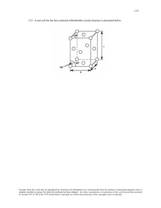
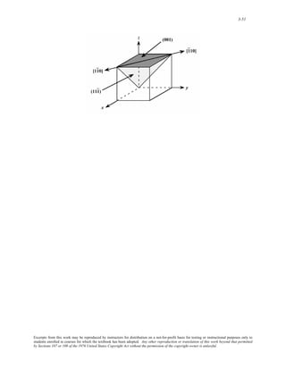
3.27 This problem calls for us to draw a [ 21 1] direction within an orthorhombic unit cell (a ≠ b ≠ c, α = β
= γ = 90°). Such a unit cell with its origin positioned at point O is shown below. We first move along the +x-axis
2a units (from point O to point A), then parallel to the +y-axis -b units (from point A to point B). Finally, we
proceed parallel to the z-axis c units (from point B to point C). The [ 21 1] direction is the vector from the origin
(point O) to point C as shown.
Excerpts from this work may be reproduced by instructors for distribution on a not-for-profit basis for testing or instructional purposes only to
students enrolled in courses for which the textbook has been adopted. Any other reproduction or translation of this work beyond that permitted
by Sections 107 or 108 of the 1976 United States Copyright Act without the permission of the copyright owner is unlawful.](https://image.slidesharecdn.com/ecyluo1ys2qvoutji72q-signature-9b381c5777758ee4fe884904ded9f35d0b251da572c8ac51c821cb24bd095f1b-poli-141018125101-conversion-gate02/85/solution-for-Materials-Science-and-Engineering-7th-edition-by-William-D-Callister-Jr-56-320.jpg)
![3-32
3.28 This problem asks that a [ 1 01] direction be drawn within a monoclinic unit cell (a ≠ b ≠ c, and α = β
= 90º ≠ γ). One such unit cell with its origin at point O is sketched below. For this direction, we move from the
origin along the minus x-axis a units (from point O to point P). There is no projection along the y-axis since the
next index is zero. Since the final index is a one, we move from point P parallel to the z-axis, c units (to point Q).
Thus, the [ 1 01] direction corresponds to the vector passing from the origin to point Q, as indicated in the figure.
Excerpts from this work may be reproduced by instructors for distribution on a not-for-profit basis for testing or instructional purposes only to
students enrolled in courses for which the textbook has been adopted. Any other reproduction or translation of this work beyond that permitted
by Sections 107 or 108 of the 1976 United States Copyright Act without the permission of the copyright owner is unlawful.](https://image.slidesharecdn.com/ecyluo1ys2qvoutji72q-signature-9b381c5777758ee4fe884904ded9f35d0b251da572c8ac51c821cb24bd095f1b-poli-141018125101-conversion-gate02/85/solution-for-Materials-Science-and-Engineering-7th-edition-by-William-D-Callister-Jr-57-320.jpg)
![3-33
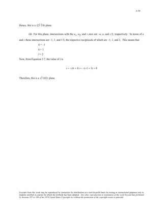
3.29 We are asked for the indices of the two directions sketched in the figure. For direction 1, the
projection on the x-axis is a, while projections on the y- and z-axes are -b/2 and -c, respectively. This is a [ 21 2 ]
direction as indicated in the summary below.
x y z
Projections a -b/2 -c
Projections in terms of a, b, and c 1 -1/2 -1
Reduction to integers 2 -1 -2
Enclosure [ 21 2 ]
Direction 2 is [102] as summarized below.
x y z
Projections a/2 0b c
Projections in terms of a, b, and c 1/2 0 1
Reduction to integers 1 0 2
Enclosure [102]
Excerpts from this work may be reproduced by instructors for distribution on a not-for-profit basis for testing or instructional purposes only to
students enrolled in courses for which the textbook has been adopted. Any other reproduction or translation of this work beyond that permitted
by Sections 107 or 108 of the 1976 United States Copyright Act without the permission of the copyright owner is unlawful.](https://image.slidesharecdn.com/ecyluo1ys2qvoutji72q-signature-9b381c5777758ee4fe884904ded9f35d0b251da572c8ac51c821cb24bd095f1b-poli-141018125101-conversion-gate02/85/solution-for-Materials-Science-and-Engineering-7th-edition-by-William-D-Callister-Jr-58-320.jpg)

![3-35
3.31 Direction A is a [ 1 10]direction, which determination is summarized as follows. We first of all
position the origin of the coordinate system at the tail of the direction vector; then in terms of this new coordinate
system
x y z
Projections – a b 0c
Projections in terms of a, b, and c –1 1 0
Reduction to integers not necessary
Enclosure [ 1 10]
Direction B is a [121] direction, which determination is summarized as follows. The vector passes through
the origin of the coordinate system and thus no translation is necessary. Therefore,
x y z
Projections
a
2
b
c
2
Projections in terms of a, b, and c
1
2
1
1
2
Reduction to integers 1 2 1
Enclosure [121]
Direction C is a [ 01 2 ] direction, which determination is summarized as follows. We first of all position
the origin of the coordinate system at the tail of the direction vector; then in terms of this new coordinate system
x y z
Projections 0a
− b
2
– c
Projections in terms of a, b, and c 0 –
1
2
–1
Reduction to integers 0 –1 –2
Enclosure [ 01 2 ]
Direction D is a [ 12 1] direction, which determination is summarized as follows. We first of all position
the origin of the coordinate system at the tail of the direction vector; then in terms of this new coordinate system
x y z
Projections
a
2
–b
c
2
Projections in terms of a, b, and c
1
2
–1
1
2
Reduction to integers 1 –2 1
Enclosure [ 12 1]
Excerpts from this work may be reproduced by instructors for distribution on a not-for-profit basis for testing or instructional purposes only to
students enrolled in courses for which the textbook has been adopted. Any other reproduction or translation of this work beyond that permitted
by Sections 107 or 108 of the 1976 United States Copyright Act without the permission of the copyright owner is unlawful.](https://image.slidesharecdn.com/ecyluo1ys2qvoutji72q-signature-9b381c5777758ee4fe884904ded9f35d0b251da572c8ac51c821cb24bd095f1b-poli-141018125101-conversion-gate02/85/solution-for-Materials-Science-and-Engineering-7th-edition-by-William-D-Callister-Jr-60-320.jpg)
![3-36
3.32 Direction A is a [ 331 ] direction, which determination is summarized as follows. We first of all
position the origin of the coordinate system at the tail of the direction vector; then in terms of this new coordinate
system
x y z
Projections a b –
c
3
Projections in terms of a, b, and c 1 1 –
1
3
Reduction to integers 3 3 –1
Enclosure [ 331 ]
Direction B is a [ 4 03 ] direction, which determination is summarized as follows. We first of all position
the origin of the coordinate system at the tail of the direction vector; then in terms of this new coordinate system
x y z
Projections –
2a
3
0b –
c
2
Projections in terms of a, b, and c –
2
3
0 –
1
2
Reduction to integers –4 0 –3
Enclosure [ 4 03 ]
Direction C is a [ 3 61] direction, which determination is summarized as follows. We first of all position
the origin of the coordinate system at the tail of the direction vector; then in terms of this new coordinate system
x y z
Projections –
a
2
b
c
6
Projections in terms of a, b, and c –
1
2
1
1
6
Reduction to integers –3 6 1
Enclosure [ 3 61]
Direction D is a [ 1 11 ] direction, which determination is summarized as follows. We first of all position
the origin of the coordinate system at the tail of the direction vector; then in terms of this new coordinate system
x y z
Projections –
a
2
b
2
–
c
2
Projections in terms of a, b, and c –
1
2
1
2
–
1
2
Reduction to integers –1 1 –1
Enclosure [ 1 11 ]
Excerpts from this work may be reproduced by instructors for distribution on a not-for-profit basis for testing or instructional purposes only to
students enrolled in courses for which the textbook has been adopted. Any other reproduction or translation of this work beyond that permitted
by Sections 107 or 108 of the 1976 United States Copyright Act without the permission of the copyright owner is unlawful.](https://image.slidesharecdn.com/ecyluo1ys2qvoutji72q-signature-9b381c5777758ee4fe884904ded9f35d0b251da572c8ac51c821cb24bd095f1b-poli-141018125101-conversion-gate02/85/solution-for-Materials-Science-and-Engineering-7th-edition-by-William-D-Callister-Jr-61-320.jpg)
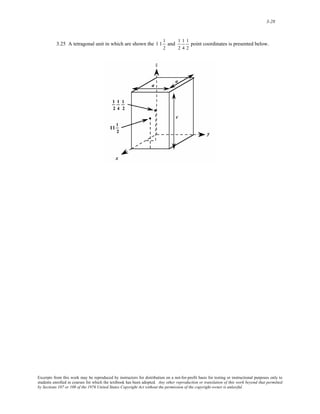
![3-37
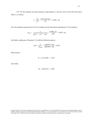
3.33 For tetragonal crystals a = b ≠ c and α = β = γ = 90°; therefore, projections along the x and y axes are
equivalent, which are not equivalent to projections along the z axis.
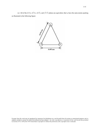
(a) Therefore, for the [011] direction, equivalent directions are the following: [101], [ 1 01 ], [ 1 01],
[ 101 ], [ 011 ] , [ 01 1] , and [ 01 1 ] .
(b) Also, for the [100] direction, equivalent directions are the following: [ 1 00] , [010], and [ 01 0].
Excerpts from this work may be reproduced by instructors for distribution on a not-for-profit basis for testing or instructional purposes only to
students enrolled in courses for which the textbook has been adopted. Any other reproduction or translation of this work beyond that permitted
by Sections 107 or 108 of the 1976 United States Copyright Act without the permission of the copyright owner is unlawful.](https://image.slidesharecdn.com/ecyluo1ys2qvoutji72q-signature-9b381c5777758ee4fe884904ded9f35d0b251da572c8ac51c821cb24bd095f1b-poli-141018125101-conversion-gate02/85/solution-for-Materials-Science-and-Engineering-7th-edition-by-William-D-Callister-Jr-62-320.jpg)
![3-38
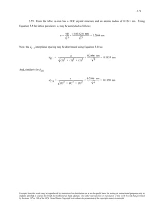
3.34 We are asked to convert [110] and [ 001 ] directions into the four-index Miller-Bravais scheme for
hexagonal unit cells. For [110]
u' = 1,
v' = 1,
w' = 0
From Equations 3.6
u = 1
3
(2uÕ− vÕ) = 1
3
[(2)(1) − 1] = 1
3
v = 1
3
(2vÕ− uÕ) = 1
3
[(2)(1) − 1] = 1
3
t = − (u + v) = − 1
3
+ 1
3
⎛
⎜
⎝
⎞
⎠
⎟ = − 2
3
w = w' = 0
It is necessary to multiply these numbers by 3 in order to reduce them to the lowest set of integers. Thus, the
direction is represented as [uvtw] = [ 112 0] .
For [ 001 ] , u' = 0, v' = 0, and w' = -1; therefore,
u = 1
3
[(2)(0) − 0] = 0
v = 1
3
[(2)(0) − 0] = 0
t = - (0 + 0) = 0
w = -1
Thus, the direction is represented as [uvtw] = [ 0001 ] .
Excerpts from this work may be reproduced by instructors for distribution on a not-for-profit basis for testing or instructional purposes only to
students enrolled in courses for which the textbook has been adopted. Any other reproduction or translation of this work beyond that permitted
by Sections 107 or 108 of the 1976 United States Copyright Act without the permission of the copyright owner is unlawful.](https://image.slidesharecdn.com/ecyluo1ys2qvoutji72q-signature-9b381c5777758ee4fe884904ded9f35d0b251da572c8ac51c821cb24bd095f1b-poli-141018125101-conversion-gate02/85/solution-for-Materials-Science-and-Engineering-7th-edition-by-William-D-Callister-Jr-63-320.jpg)
![3-39
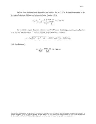
3.35 This problem asks for the determination of indices for several directions in a hexagonal unit cell.
For direction A, projections on the a1, a2, and z axes are –a, –a, and c, or, in terms of a and c the
projections are –1, –1, and 1. This means that
u’ = –1
v’ = –1
w’ = 1
Now, from Equations 3.6, the u, v, t, and w indices become
u = 1
3
(2u' − v' ) = 1
3
[(2)(−1) − (−1)] = − 1
3
v = 1
3
(2vÕ− uÕ) = 1
3
[(2)(−1) − (−1)] = − 1
3
t = − (u + v) = − − 1
3
− 1
3
⎛
⎜
⎝
⎞
⎠
⎟ = 2
3
w = w’ = 1
Now, in order to get the lowest set of integers, it is necessary to multiply all indices by the factor 3, with the result
that the direction A is a [ 1 1 23] direction.
For direction B, projections on the a1, a2, and z axes are –a, 0a, and 0c, or, in terms of a and c the
projections are –1, 0, and 0. This means that
u’ = –1
v’ = 0
w’ = 0
Now, from Equations 3.6, the u, v, t, and w indices become
u = 1
3
(2u' − v) = 1
3
[(2)(−1) − 0] = − 2
3
v = 1
3
(2v' − u' ) = 1
3
[(2)(0) − (−1)] = 1
3
t = − (u+ v) = − − 2
3
+ 1
3
⎛
⎜
⎝
⎞
⎠
⎟ = 1
3
w = w' = 0
Excerpts from this work may be reproduced by instructors for distribution on a not-for-profit basis for testing or instructional purposes only to
students enrolled in courses for which the textbook has been adopted. Any other reproduction or translation of this work beyond that permitted
by Sections 107 or 108 of the 1976 United States Copyright Act without the permission of the copyright owner is unlawful.](https://image.slidesharecdn.com/ecyluo1ys2qvoutji72q-signature-9b381c5777758ee4fe884904ded9f35d0b251da572c8ac51c821cb24bd095f1b-poli-141018125101-conversion-gate02/85/solution-for-Materials-Science-and-Engineering-7th-edition-by-William-D-Callister-Jr-64-320.jpg)
![3-40
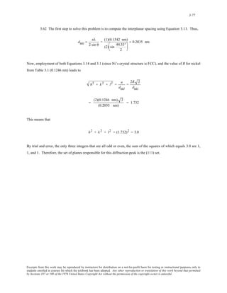
Now, in order to get the lowest set of integers, it is necessary to multiply all indices by the factor 3, with the result
that the direction B is a [ 2 110] direction.
For direction C projections on the a1, a2, and z axes are a, a/2, and 0c, or, in terms of a and c the
projections are 1, 1/2, and 0, which when multiplied by the factor 2 become the smallest set of integers: 2, 1, and 0.
This means that
u’ = 2
v’ = 1
w’ = 0
Now, from Equations 3.6, the u, v, t, and w indices become
u = 1
3
(2uÕ− v) = 1
3
[(2)(2) −1] = 3
3
= 1
v = 1
3
(2vÕ− uÕ) = 1
3
[(2)(1) − 2] = 0
t = − (u+ v) = −(1 − 0) = −1
w = w' = 0
No reduction is necessary inasmuch as all the indices are integers. Therefore, direction C is a [ 101 0] .
For direction D projections on the a1, a2, and z axes are a, 0a, and c/2, or, in terms of a and c the
projections are 1, 0, and 1/2, which when multiplied by the factor 2 become the smallest set of integers: 2, 0, and 1.
This means that
u’ = 2
v’ = 0
w’ = 1
Now, from Equations 3.6, the u, v, t, and w indices become
u = 1
3
(2u' − v' ) = 1
3
[(2)(2) − 0] = 4
3
v = 1
3
(2vÕ− uÕ) = 1
3
[(2)(0) − (2)] =− 2
3
Excerpts from this work may be reproduced by instructors for distribution on a not-for-profit basis for testing or instructional purposes only to
students enrolled in courses for which the textbook has been adopted. Any other reproduction or translation of this work beyond that permitted
by Sections 107 or 108 of the 1976 United States Copyright Act without the permission of the copyright owner is unlawful.](https://image.slidesharecdn.com/ecyluo1ys2qvoutji72q-signature-9b381c5777758ee4fe884904ded9f35d0b251da572c8ac51c821cb24bd095f1b-poli-141018125101-conversion-gate02/85/solution-for-Materials-Science-and-Engineering-7th-edition-by-William-D-Callister-Jr-65-320.jpg)
![3-42
3.36 This problem asks for us to derive expressions for each of the three primed indices in terms of the
four unprimed indices.
It is first necessary to do an expansion of Equation 3.6a as
u = 1
3
(2u' − v) = 2u'
3
− v'
3
And solving this expression for v’ yields
v' = 2u' − 3u
Now, substitution of this expression into Equation 3.6b gives
v = 1
3
(2vÕ− uÕ) = 1
3
[(2)(2uÕ− 3u) − uÕ] = uÕ− 2u
Or
u' = v + 2u
And, solving for v from Equation 3.6c leads to
v = − (u + t)
which, when substituted into the above expression for u’ yields
u' = v + 2u = − u − t + 2u = u − t
In solving for an expression for v’, we begin with the one of the above expressions for this parameter—i.e.,
v' = 2u' − 3u
Now, substitution of the above expression for u’ into this equation leads to
vÕ= 2uÕ− 3u = (2)(u − t) − 3u = − u −2t
And solving for u from Equation 3.6c gives
Excerpts from this work may be reproduced by instructors for distribution on a not-for-profit basis for testing or instructional purposes only to
students enrolled in courses for which the textbook has been adopted. Any other reproduction or translation of this work beyond that permitted
by Sections 107 or 108 of the 1976 United States Copyright Act without the permission of the copyright owner is unlawful.](https://image.slidesharecdn.com/ecyluo1ys2qvoutji72q-signature-9b381c5777758ee4fe884904ded9f35d0b251da572c8ac51c821cb24bd095f1b-poli-141018125101-conversion-gate02/85/solution-for-Materials-Science-and-Engineering-7th-edition-by-William-D-Callister-Jr-66-320.jpg)


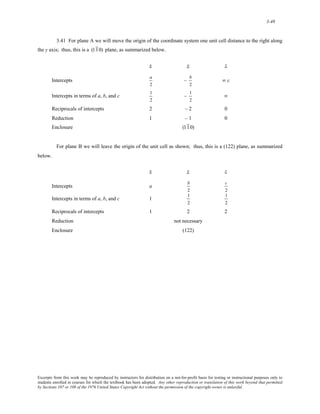
![3-47
3.40 For plane A we will leave the origin at the unit cell as shown. If we extend this plane back into the
plane of the page, then it is a (111 ) plane, as summarized below.
x y z
Intercepts a b – c
Intercepts in terms of a, b, and c 1 1 – 1
Reciprocals of intercepts 1 1 – 1
Reduction not necessary
Enclosure (111 )
[Note: If we move the origin one unit cell distance parallel to the x axis and then one unit cell distance parallel to
the y axis, the direction becomes (1 1 1) ].
For plane B we will leave the origin of the unit cell as shown; this is a (230) plane, as summarized below.
x y z
Intercepts
a
2
b
3
∞c
Intercepts in terms of a, b, and c
1
2
1
3
∞
Reciprocals of intercepts 2 3 0
Enclosure (230)
Excerpts from this work may be reproduced by instructors for distribution on a not-for-profit basis for testing or instructional purposes only to
students enrolled in courses for which the textbook has been adopted. Any other reproduction or translation of this work beyond that permitted
by Sections 107 or 108 of the 1976 United States Copyright Act without the permission of the copyright owner is unlawful.](https://image.slidesharecdn.com/ecyluo1ys2qvoutji72q-signature-9b381c5777758ee4fe884904ded9f35d0b251da572c8ac51c821cb24bd095f1b-poli-141018125101-conversion-gate02/85/solution-for-Materials-Science-and-Engineering-7th-edition-by-William-D-Callister-Jr-71-320.jpg)
![3-41
t = − (u+ v) = − 4
3
− 2
3
⎛
⎜
⎝
⎞
⎠
⎟ = − 2
3
w = w' = 1
Now, in order to get the lowest set of integers, it is necessary to multiply all indices by the factor 3, with the result
that the direction D is a [ 42 2 3] direction.
Excerpts from this work may be reproduced by instructors for distribution on a not-for-profit basis for testing or instructional purposes only to
students enrolled in courses for which the textbook has been adopted. Any other reproduction or translation of this work beyond that permitted
by Sections 107 or 108 of the 1976 United States Copyright Act without the permission of the copyright owner is unlawful.](https://image.slidesharecdn.com/ecyluo1ys2qvoutji72q-signature-9b381c5777758ee4fe884904ded9f35d0b251da572c8ac51c821cb24bd095f1b-poli-141018125101-conversion-gate02/85/solution-for-Materials-Science-and-Engineering-7th-edition-by-William-D-Callister-Jr-73-320.jpg)

![3-50
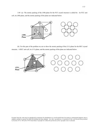
3.43 (a) In the figure below is shown (110) and (111) planes, and, as indicated, their intersection results in a
[ 1 10] , or equivalently, a [ 11 0] direction.
(b) In the figure below is shown (110) and (11 0) planes, and, as indicated, their intersection results in a
[001], or equivalently, a [ 001 ] direction.
(c) In the figure below is shown (111 ) and (001) planes, and, as indicated, their intersection results in a
[ 1 10] , or equivalently, a [ 11 0] direction.
Excerpts from this work may be reproduced by instructors for distribution on a not-for-profit basis for testing or instructional purposes only to
students enrolled in courses for which the textbook has been adopted. Any other reproduction or translation of this work beyond that permitted
by Sections 107 or 108 of the 1976 United States Copyright Act without the permission of the copyright owner is unlawful.](https://image.slidesharecdn.com/ecyluo1ys2qvoutji72q-signature-9b381c5777758ee4fe884904ded9f35d0b251da572c8ac51c821cb24bd095f1b-poli-141018125101-conversion-gate02/85/solution-for-Materials-Science-and-Engineering-7th-edition-by-William-D-Callister-Jr-75-320.jpg)
![3-53
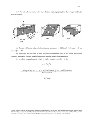
3.45 (a) The unit cell in Problem 3.20 is body-centered tetragonal. Of the three planes given in the
problem statement the (100) and (01 0) are equivalent—that is, have the same atomic packing. The atomic packing
for these two planes as well as the (001) are shown in the figure below.
(b) Of the four planes cited in the problem statement, only (101), (011), and (1 01) are equivalent—have
the same atomic packing. The atomic arrangement of these planes as well as the (110) are presented in the figure
below. Note: the 0.495 nm dimension for the (110) plane comes from the relationship
[(nm)2 (1 /2
0.35 + 0.35 nm)2 ] . Likewise, the 0.570 nm dimension for the (101), (011), and (1 01) planes comes
from
[(0.35 nm)2 + (0.45 nm)2]1/2
.
Excerpts from this work may be reproduced by instructors for distribution on a not-for-profit basis for testing or instructional purposes only to
students enrolled in courses for which the textbook has been adopted. Any other reproduction or translation of this work beyond that permitted
by Sections 107 or 108 of the 1976 United States Copyright Act without the permission of the copyright owner is unlawful.](https://image.slidesharecdn.com/ecyluo1ys2qvoutji72q-signature-9b381c5777758ee4fe884904ded9f35d0b251da572c8ac51c821cb24bd095f1b-poli-141018125101-conversion-gate02/85/solution-for-Materials-Science-and-Engineering-7th-edition-by-William-D-Callister-Jr-78-320.jpg)

![3-57
3.48 This problem asks that we convert (111) and (01 2) planes into the four-index Miller-Bravais
scheme, (hkil), for hexagonal cells. For (111), h = 1, k = 1, and l = 1, and, from Equation 3.7, the value of i is equal
to
i = − (h + k) = − (1 + 1) = − 2
Therefore, the (111) plane becomes (112 1) .
Now for the (01 2) plane, h = 0, k = -1, and l = 2, and computation of i using Equation 3.7 leads to
i = − (h + k) = −[0 + (−1)] = 1
such that (01 2) becomes (01 12) .
Excerpts from this work may be reproduced by instructors for distribution on a not-for-profit basis for testing or instructional purposes only to
students enrolled in courses for which the textbook has been adopted. Any other reproduction or translation of this work beyond that permitted
by Sections 107 or 108 of the 1976 United States Copyright Act without the permission of the copyright owner is unlawful.](https://image.slidesharecdn.com/ecyluo1ys2qvoutji72q-signature-9b381c5777758ee4fe884904ded9f35d0b251da572c8ac51c821cb24bd095f1b-poli-141018125101-conversion-gate02/85/solution-for-Materials-Science-and-Engineering-7th-edition-by-William-D-Callister-Jr-82-320.jpg)
![3-58
3.49 This problem asks for the determination of Bravais-Miller indices for several planes in hexagonal
unit cells.
(a) For this plane, intersections with the a1, a2, and z axes are ∞a, –a, and ∞c (the plane parallels both a1
and z axes). In terms of a and c these intersections are ∞, –1, and ∞, the respective reciprocals of which are 0, –1,
and 0. This means that
h = 0
k = –1
l = 0
Now, from Equation 3.7, the value of i is
i = − (h + k) = −[0 + (−1)] = 1
Hence, this is a (01 10) plane.
(b) For this plane, intersections with the a1, a2, and z axes are –a, –a, and c/2, respectively. In terms of a
and c these intersections are –1, –1, and 1/2, the respective reciprocals of which are –1, –1, and 2. This means that
h = –1
k = –1
l = 2
Now, from Equation 3.7, the value of i is
i = − (h + k) = − (−1 − 1) = 2
Hence, this is a (1 1 22) plane.
(c) For this plane, intersections with the a1, a2, and z axes are a/2, –a, and ∞c (the plane parallels the z
axis). In terms of a and c these intersections are 1/2, –1, and ∞, the respective reciprocals of which are 2, –1, and 0.
This means that
h = 2
k = –1
l = 0
Now, from Equation 3.7, the value of i is
i = − (h + k) = − (2 − 1) = −1
Excerpts from this work may be reproduced by instructors for distribution on a not-for-profit basis for testing or instructional purposes only to
students enrolled in courses for which the textbook has been adopted. Any other reproduction or translation of this work beyond that permitted
by Sections 107 or 108 of the 1976 United States Copyright Act without the permission of the copyright owner is unlawful.](https://image.slidesharecdn.com/ecyluo1ys2qvoutji72q-signature-9b381c5777758ee4fe884904ded9f35d0b251da572c8ac51c821cb24bd095f1b-poli-141018125101-conversion-gate02/85/solution-for-Materials-Science-and-Engineering-7th-edition-by-William-D-Callister-Jr-83-320.jpg)

![3-61
Linear and Planar Densities
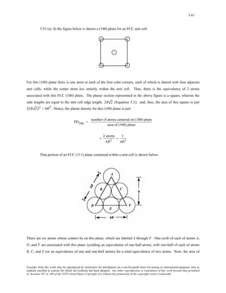
3.51 (a) In the figure below is shown a [100] direction within an FCC unit cell.
For this [100] direction there is one atom at each of the two unit cell corners, and, thus, there is the equivalent of 1
atom that is centered on the direction vector. The length of this direction vector is just the unit cell edge length,
2R 2 (Equation 3.1). Therefore, the expression for the linear density of this plane is
LD100 = number of atoms centered on [100] direction vector
length of [100] direction vector
= 1 atom
2R 2
= 1
2R 2
An FCC unit cell within which is drawn a [111] direction is shown below.
For this [111] direction, the vector shown passes through only the centers of the single atom at each of its ends, and,
thus, there is the equivalence of 1 atom that is centered on the direction vector. The length of this direction vector is
denoted by z in this figure, which is equal to
z = x2 + y2
Excerpts from this work may be reproduced by instructors for distribution on a not-for-profit basis for testing or instructional purposes only to
students enrolled in courses for which the textbook has been adopted. Any other reproduction or translation of this work beyond that permitted
by Sections 107 or 108 of the 1976 United States Copyright Act without the permission of the copyright owner is unlawful.](https://image.slidesharecdn.com/ecyluo1ys2qvoutji72q-signature-9b381c5777758ee4fe884904ded9f35d0b251da572c8ac51c821cb24bd095f1b-poli-141018125101-conversion-gate02/85/solution-for-Materials-Science-and-Engineering-7th-edition-by-William-D-Callister-Jr-86-320.jpg)
![3-62
where x is the length of the bottom face diagonal, which is equal to 4R. Furthermore, y is the unit cell edge length,
which is equal to 2R 2 (Equation 3.1). Thus, using the above equation, the length z may be calculated as follows:
z = (4R)2 + (2R 2)2 = 24R2 = 2 R 6
Therefore, the expression for the linear density of this direction is
LD111 = number of atoms centered on [111] direction vector
length of [111] direction vector
= 1 atom
2 R 6
= 1
2 R 6
(b) From the table inside the front cover, the atomic radius for copper is 0.128 nm. Therefore, the linear
density for the [100] direction is
LD100 (Cu) = 1
2 R 2
= 1
(2)(0.128 nm) 2
= 2.76 nm−1 = 2.76 × 10⁹ m−1
While for the [111] direction
LD111(Cu) = 1
2R 6
= 1
(2)(0.128 nm) 6
= 1.59 nm−1 = 1.59 × 10⁹ m−1
Excerpts from this work may be reproduced by instructors for distribution on a not-for-profit basis for testing or instructional purposes only to
students enrolled in courses for which the textbook has been adopted. Any other reproduction or translation of this work beyond that permitted
by Sections 107 or 108 of the 1976 United States Copyright Act without the permission of the copyright owner is unlawful.](https://image.slidesharecdn.com/ecyluo1ys2qvoutji72q-signature-9b381c5777758ee4fe884904ded9f35d0b251da572c8ac51c821cb24bd095f1b-poli-141018125101-conversion-gate02/85/solution-for-Materials-Science-and-Engineering-7th-edition-by-William-D-Callister-Jr-87-320.jpg)
![3-63
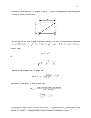
3.52 (a) In the figure below is shown a [110] direction within a BCC unit cell.
For this [110] direction there is one atom at each of the two unit cell corners, and, thus, there is the equivalence of 1
atom that is centered on the direction vector. The length of this direction vector is denoted by x in this figure, which
is equal to
x = z 2 − y2
where y is the unit cell edge length, which, from Equation 3.3 is equal to
4R
3
. Furthermore, z is the length of the
unit cell diagonal, which is equal to 4R Thus, using the above equation, the length x may be calculated as follows:
x = (4R)2 − 4R
3
⎛
⎜⎜
⎝
⎞
⎟⎟
⎠
2
= 32R2
3
= 4R 2
3
Therefore, the expression for the linear density of this direction is
LD110 = number of atoms centered on [110] direction vector
length of [110] direction vector
= 1 atom
4R 2
3
=
3
4 R 2
A BCC unit cell within which is drawn a [111] direction is shown below.
Excerpts from this work may be reproduced by instructors for distribution on a not-for-profit basis for testing or instructional purposes only to
students enrolled in courses for which the textbook has been adopted. Any other reproduction or translation of this work beyond that permitted
by Sections 107 or 108 of the 1976 United States Copyright Act without the permission of the copyright owner is unlawful.](https://image.slidesharecdn.com/ecyluo1ys2qvoutji72q-signature-9b381c5777758ee4fe884904ded9f35d0b251da572c8ac51c821cb24bd095f1b-poli-141018125101-conversion-gate02/85/solution-for-Materials-Science-and-Engineering-7th-edition-by-William-D-Callister-Jr-88-320.jpg)
![3-64
For although the [111] direction vector shown passes through the centers of three atoms, there is an equivalence of
only two atoms associated with this unit cell—one-half of each of the two atoms at the end of the vector, in addition
to the center atom belongs entirely to the unit cell. Furthermore, the length of the vector shown is equal to 4R, since
all of the atoms whose centers the vector passes through touch one another. Therefore, the linear density is equal to
LD111 = number of atoms centered on [111] direction vector
length of [111] direction vector
= 2 atoms
4R
= 1
2R
(b) From the table inside the front cover, the atomic radius for iron is 0.124 nm. Therefore, the linear
density for the [110] direction is
LD110 (Fe) =
3
4 R 2
=
3
(4)(0.124 nm) 2
= 2.47 nm−1 = 2.47 × 10⁹ m−1
While for the [111] direction
LD111(Fe) = 1
2R
= 1
(2)(0.124 nm)
= 4.03 nm−1 = 4.03 × 10⁹ m−1
Excerpts from this work may be reproduced by instructors for distribution on a not-for-profit basis for testing or instructional purposes only to
students enrolled in courses for which the textbook has been adopted. Any other reproduction or translation of this work beyond that permitted
by Sections 107 or 108 of the 1976 United States Copyright Act without the permission of the copyright owner is unlawful.](https://image.slidesharecdn.com/ecyluo1ys2qvoutji72q-signature-9b381c5777758ee4fe884904ded9f35d0b251da572c8ac51c821cb24bd095f1b-poli-141018125101-conversion-gate02/85/solution-for-Materials-Science-and-Engineering-7th-edition-by-William-D-Callister-Jr-89-320.jpg)


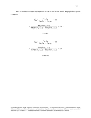
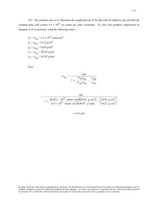
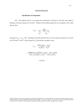
![4-11
ρave =
m1 + m2
V1 + V2
[Note: here it is assumed that the total alloy volume is equal to the separate volumes of the individual components,
which is only an approximation; normally V will not be exactly equal to (V1 + V2)].
Each of V1 and V2 may be expressed in terms of its mass and density as,
V1 =
m1
ρ1
V2 =
m2
ρ2
When these expressions are substituted into the above equation, we get
ρave =
m1 + m2
m1
+
ρ1
m2
ρ2
Furthermore, from Equation 4.3
m1 =
C1 (m1 + m2)
100
m2 =
C2 (m1 + m2)
100
Which, when substituted into the above ρave expression yields
ρave =
m1 + m2
C1 (m1 + m2)
100
ρ1
+
C2 (m1 + m2)
100
ρ2
And, finally, this equation reduces to
= 100
C1
+
ρ1
C2
ρ2
Excerpts from this work may be reproduced by instructors for distribution on a not-for-profit basis for testing or instructional purposes only to
students enrolled in courses for which the textbook has been adopted. Any other reproduction or translation of this work beyond that permitted
by Sections 107 or 108 of the 1976 United States Copyright Act without the permission of the copyright owner is unlawful.](https://image.slidesharecdn.com/ecyluo1ys2qvoutji72q-signature-9b381c5777758ee4fe884904ded9f35d0b251da572c8ac51c821cb24bd095f1b-poli-141018125101-conversion-gate02/85/solution-for-Materials-Science-and-Engineering-7th-edition-by-William-D-Callister-Jr-117-320.jpg)


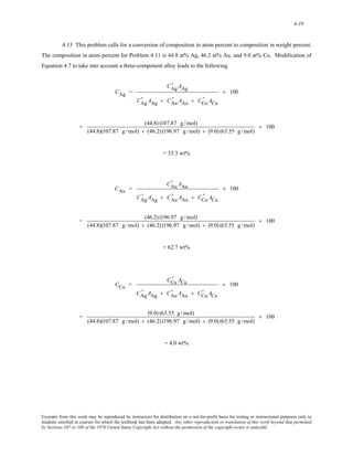


![4-37
Interfacial Defects
4.27 The surface energy for a crystallographic plane will depend on its packing density [i.e., the planar
density (Section 3.11)]—that is, the higher the packing density, the greater the number of nearest-neighbor atoms,
and the more atomic bonds in that plane that are satisfied, and, consequently, the lower the surface energy. From
the solution to Problem 3.53, planar densities for FCC (100) and (111) planes are 1
4R2 and 1
2R2 3
, respectively—
that is 0.25
R2 and 0.29
R2 (where R is the atomic radius). Thus, since the planar density for (111) is greater, it will have
the lower surface energy.
Excerpts from this work may be reproduced by instructors for distribution on a not-for-profit basis for testing or instructional purposes only to
students enrolled in courses for which the textbook has been adopted. Any other reproduction or translation of this work beyond that permitted
by Sections 107 or 108 of the 1976 United States Copyright Act without the permission of the copyright owner is unlawful.](https://image.slidesharecdn.com/ecyluo1ys2qvoutji72q-signature-9b381c5777758ee4fe884904ded9f35d0b251da572c8ac51c821cb24bd095f1b-poli-141018125101-conversion-gate02/85/solution-for-Materials-Science-and-Engineering-7th-edition-by-William-D-Callister-Jr-142-320.jpg)
![4-38
4.28 The surface energy for a crystallographic plane will depend on its packing density [i.e., the planar
density (Section 3.11)]—that is, the higher the packing density, the greater the number of nearest-neighbor atoms,
and the more atomic bonds in that plane that are satisfied, and, consequently, the lower the surface energy. From
the solution to Problem 3.54, the planar densities for BCC (100) and (110) are 3
16R2 and 3
8R2 2
, respectively—
that is 0.19
R2 and 0.27
R2 . Thus, since the planar density for (110) is greater, it will have the lower surface energy.
Excerpts from this work may be reproduced by instructors for distribution on a not-for-profit basis for testing or instructional purposes only to
students enrolled in courses for which the textbook has been adopted. Any other reproduction or translation of this work beyond that permitted
by Sections 107 or 108 of the 1976 United States Copyright Act without the permission of the copyright owner is unlawful.](https://image.slidesharecdn.com/ecyluo1ys2qvoutji72q-signature-9b381c5777758ee4fe884904ded9f35d0b251da572c8ac51c821cb24bd095f1b-poli-141018125101-conversion-gate02/85/solution-for-Materials-Science-and-Engineering-7th-edition-by-William-D-Callister-Jr-143-320.jpg)


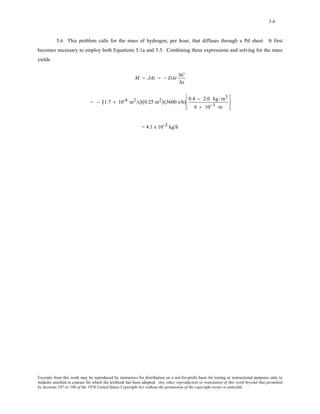

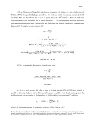
![5-9
5.9 This problems asks for us to compute the diffusion flux of nitrogen gas through a 1.5-mm thick plate
of iron at 300°C when the pressures on the two sides are 0.10 and 5.0 MPa. Ultimately we will employ Equation
5.3 to solve this problem. However, it first becomes necessary to determine the concentration of hydrogen at each
face using Equation 5.11. At the low pressure (or B) side
CN(B) = (4.90 × 10⁻³) 0.10 MPa exp − 37,600 J /mol
(8.31 J /mol - K)(300 + 273 K)
⎡
⎢⎣
⎤
⎥⎦
5.77 x 10⁻⁷ wt%
Whereas, for the high pressure (or A) side
CN(A) = (4.90 × 10⁻³) 5.0 MPa exp − 37,600 J /mol
(8.31 J /mol - K)(300 + 273 K)
⎡
⎢⎣
⎤
⎥⎦
4.08 x 10⁻⁶ wt%
We now convert concentrations in weight percent to mass of nitrogen per unit volume of solid. At face B there are
5.77 x 10⁻⁷ g (or 5.77 x 10⁻¹⁰ kg) of hydrogen in 100 g of Fe, which is virtually pure iron. From the density of iron
(7.87 g/cm3), the volume iron in 100 g (VB) is just
VB = 100 g
7.87 g /cm3 = 12.7 cm3 = 1.27 × 10⁻⁵ m3
''
Therefore, the concentration of hydrogen at the B face in kilograms of N per cubic meter of alloy [CN(B)] is just
'' =
CN(B)
CN(B)
VB
= 5.77 × 10⁻¹⁰ kg
1.27 × 10⁻⁵ m3 = 4.54 x 10⁻⁵ kg/m3
At the A face the volume of iron in 100 g (VA) will also be 1.27 x 10⁻⁵ m3, and
'' =
CN(A)
CN(A)
VA
Excerpts from this work may be reproduced by instructors for distribution on a not-for-profit basis for testing or instructional purposes only to
students enrolled in courses for which the textbook has been adopted. Any other reproduction or translation of this work beyond that permitted
by Sections 107 or 108 of the 1976 United States Copyright Act without the permission of the copyright owner is unlawful.](https://image.slidesharecdn.com/ecyluo1ys2qvoutji72q-signature-9b381c5777758ee4fe884904ded9f35d0b251da572c8ac51c821cb24bd095f1b-poli-141018125101-conversion-gate02/85/solution-for-Materials-Science-and-Engineering-7th-edition-by-William-D-Callister-Jr-163-320.jpg)


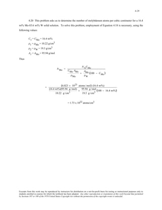
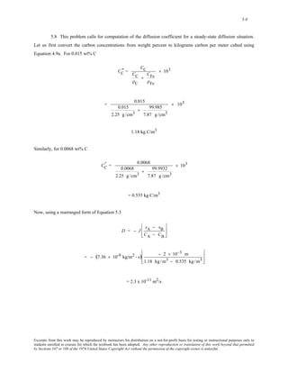
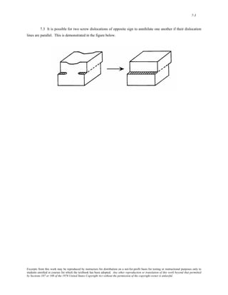
![5-23
5.18 We are asked to calculate the temperature at which the diffusion coefficient for the diffusion of Zn in
Cu has a value of 2.6 x 10⁻¹⁶ m2/s. Solving for T from Equation 5.9a
T = −
Qd
R(ln D − ln D0)
and using the data from Table 5.2 for the diffusion of Zn in Cu (i.e., D0 = 2.4 x 10⁻⁵ m2/s and Qd = 189,000 J/mol) ,
we get
T = − 189,000 J/mol
(8.31 J/mol - K) ln ([ 2.6 × 10 -16 m2/s) − ln (2.4 × 10 -5 m2/s) ]
= 901 K = 628°C
Note: this problem may also be solved using the “Diffusion” module in the VMSE software. Open the “Diffusion”
module, click on the “D vs 1/T Plot” submodule, and then do the following:
1. In the left-hand window that appears, there is a preset set of data for the diffusion of Zn in Cu system.
However, the temperature range does not extend to conditions specified in the problem statement. Thus, this
requires us specify our settings by clicking on the “Custom1” box.
2. In the column on the right-hand side of this window enter the data for this problem. In the window
under “D0” enter preexponential value from Table 5.2—viz. “2.4e-5”. Next just below the “Qd” window enter the
activation energy value—viz. “189”. It is next necessary to specify a temperature range over which the data is to be
plotted. The temperature at which D has the stipulated value is probably between 500ºC and 1000ºC, so enter “500”
in the “T Min” box that is beside “C”; and similarly for the maximum temperature—enter “1000” in the box below
“T Max”.
3. Next, at the bottom of this window, click the “Add Curve” button.
4. A log D versus 1/T plot then appears, with a line for the temperature dependence of the diffusion
coefficient for Zn in Cu. At the top of this curve is a diamond-shaped cursor. Click-and-drag this cursor down the
line to the point at which the entry under the “Diff Coeff (D):” label reads 2.6 x 10⁻¹⁶ m2/s. The temperature at
which the diffusion coefficient has this value is given under the label “Temperature (T):”. For this problem, the
value is 903 K.
Excerpts from this work may be reproduced by instructors for distribution on a not-for-profit basis for testing or instructional purposes only to
students enrolled in courses for which the textbook has been adopted. Any other reproduction or translation of this work beyond that permitted
by Sections 107 or 108 of the 1976 United States Copyright Act without the permission of the copyright owner is unlawful.](https://image.slidesharecdn.com/ecyluo1ys2qvoutji72q-signature-9b381c5777758ee4fe884904ded9f35d0b251da572c8ac51c821cb24bd095f1b-poli-141018125101-conversion-gate02/85/solution-for-Materials-Science-and-Engineering-7th-edition-by-William-D-Callister-Jr-177-320.jpg)
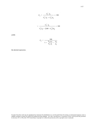
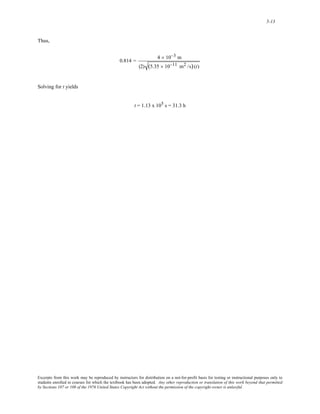
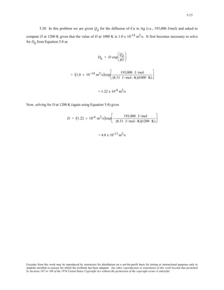
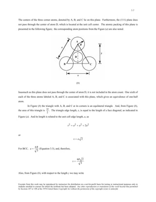
![5-24
5.19 For this problem we are given D0 (1.1 x 10⁻⁴) and Qd (272,000 J/mol) for the diffusion of Cr in Ni,
and asked to compute the temperature at which D = 1.2 x 10⁻¹⁴ m2/s. Solving for T from Equation 5.9a yields
T =
Qd
R(ln D0 − ln D)
= 272,000 J/mol
(8.31 J/mol - K) ln ([ 1.1 × 10⁻⁴ m2/s) - ln (1.2 × 10⁻¹⁴ m2/s)]
= 1427 K = 1154°C
Note: this problem may also be solved using the “Diffusion” module in the VMSE software. Open the “Diffusion”
module, click on the “D vs 1/T Plot” submodule, and then do the following:
1. In the left-hand window that appears, click on the “Custom1” box.
2. In the column on the right-hand side of this window enter the data for this problem. In the window
under “D0” enter preexponential value—viz. “1.1e-4”. Next just below the “Qd” window enter the activation
energy value—viz. “272”. It is next necessary to specify a temperature range over which the data is to be plotted.
The temperature at which D has the stipulated value is probably between 1000ºC and 1500ºC, so enter “1000” in the
“T Min” box that is beside “C”; and similarly for the maximum temperature—enter “1500” in the box below “T
Max”.
3. Next, at the bottom of this window, click the “Add Curve” button.
4. A log D versus 1/T plot then appears, with a line for the temperature dependence of the diffusion
coefficient for Cr in Ni. At the top of this curve is a diamond-shaped cursor. Click-and-drag this cursor down the
line to the point at which the entry under the “Diff Coeff (D):” label reads 1.2 x 10⁻¹⁴ m2/s. The temperature at
which the diffusion coefficient has this value is given under the label “Temperature (T):”. For this problem, the
value is 1430 K.
Excerpts from this work may be reproduced by instructors for distribution on a not-for-profit basis for testing or instructional purposes only to
students enrolled in courses for which the textbook has been adopted. Any other reproduction or translation of this work beyond that permitted
by Sections 107 or 108 of the 1976 United States Copyright Act without the permission of the copyright owner is unlawful.](https://image.slidesharecdn.com/ecyluo1ys2qvoutji72q-signature-9b381c5777758ee4fe884904ded9f35d0b251da572c8ac51c821cb24bd095f1b-poli-141018125101-conversion-gate02/85/solution-for-Materials-Science-and-Engineering-7th-edition-by-William-D-Callister-Jr-178-320.jpg)
![5-26
5.21 (a) Using Equation 5.9a, we set up two simultaneous equations with Qd and D0 as unknowns as
follows:
ln D1 = lnD0 −
Qd
R
1
T1
⎛
⎜⎜
⎝
⎞
⎟⎟
⎠
ln D2 = lnD0 −
Qd
R
1
T2
⎛
⎜⎜
⎝
⎞
⎟⎟
⎠
Now, solving for Qd in terms of temperatures T1 and T2 (1473 K and 1673 K) and D1 and D2 (2.2 x 10⁻¹⁵ and 4.8 x
10-14 m2/s), we get
Qd = − R
ln D1 − ln D2
1
T1
− 1
T2
= − (8.31 J/mol - K)
[ln (2.2 × 10 -15) − ln (4.8 × 10 -14)]
1
1473 K
− 1
1673 K
= 315,700 J/mol
Now, solving for D0 from Equation 5.8 (and using the 1473 K value of D)
D0 = D1 exp
Qd
RT1
⎛
⎜⎜
⎝
⎞
⎟⎟
⎠
= (2.2 × 10⁻¹⁵ m2/s)exp 315,700 J /mol
(8.31 J /mol - K)(1473 K)
⎡
⎢⎣
⎤
⎥⎦
= 3.5 x 10⁻⁴ m2/s
(b) Using these values of D0 and Qd, D at 1573 K is just
D = (3.5 × 10⁻⁴ m2/s)exp − 315,700 J /mol
(8.31 J /mol - K)(1573 K)
⎡
⎢⎣
⎤
⎦⎥
Excerpts from this work may be reproduced by instructors for distribution on a not-for-profit basis for testing or instructional purposes only to
students enrolled in courses for which the textbook has been adopted. Any other reproduction or translation of this work beyond that permitted
by Sections 107 or 108 of the 1976 United States Copyright Act without the permission of the copyright owner is unlawful.](https://image.slidesharecdn.com/ecyluo1ys2qvoutji72q-signature-9b381c5777758ee4fe884904ded9f35d0b251da572c8ac51c821cb24bd095f1b-poli-141018125101-conversion-gate02/85/solution-for-Materials-Science-and-Engineering-7th-edition-by-William-D-Callister-Jr-180-320.jpg)

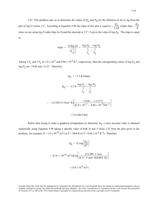
![5-28
5.22 (a) Using Equation 5.9a, we set up two simultaneous equations with Qd and D0 as unknowns as
follows:
ln D1 = lnD0 −
Qd
R
1
T1
⎛
⎜⎜
⎝
⎞
⎟⎟
⎠
ln D2 = lnD0 −
Qd
R
1
T2
⎛
⎜⎜
⎝
⎞
⎟⎟
⎠
Solving for Qd in terms of temperatures T1 and T2 (873 K [600°C] and 973 K [700°C]) and D1 and D2 (5.5 x 10⁻¹⁴
and 3.9 x 10⁻¹³ m2/s), we get
Qd = − R
ln D1 − ln D2
1
T1
− 1
T2
= −
(8.31 J/mol - K)[ln (5.5 × 10 -14) − ln (3.9 × 10 -13)]
1
873 K
− 1
973 K
= 138,300 J/mol
Now, solving for D0 from Equation 5.8 (and using the 600°C value of D)
D0 = D1 exp
Qd
RT1
⎛
⎜⎜
⎝
⎞
⎟⎟
⎠
= (5.5 × 10⁻¹⁴ m2/s)exp 138,300 J /mol
(8.31 J /mol - K)(873 K)
⎡
⎢⎣
⎤
⎥⎦
= 1.05 x 10⁻⁵ m2/s
(b) Using these values of D0 and Qd, D at 1123 K (850°C) is just
D = (1.05 × 10⁻⁵ m2/s)exp − 138,300 J /mol
(8.31 J /mol - K)(1123 K)
⎡
⎢⎣
⎤
⎥⎦
Excerpts from this work may be reproduced by instructors for distribution on a not-for-profit basis for testing or instructional purposes only to
students enrolled in courses for which the textbook has been adopted. Any other reproduction or translation of this work beyond that permitted
by Sections 107 or 108 of the 1976 United States Copyright Act without the permission of the copyright owner is unlawful.](https://image.slidesharecdn.com/ecyluo1ys2qvoutji72q-signature-9b381c5777758ee4fe884904ded9f35d0b251da572c8ac51c821cb24bd095f1b-poli-141018125101-conversion-gate02/85/solution-for-Materials-Science-and-Engineering-7th-edition-by-William-D-Callister-Jr-182-320.jpg)


![5-33
5.26 To solve this problem it is necessary to employ Equation 5.7
Dt = constant
Which, for this problem, takes the form
D1000t1000 = DTtT
At 1000°C, and using the data from Table 5.2, for the diffusion of carbon in γ-iron—i.e.,
D0 = 2.3 x 10⁻⁵ m2/s
Qd = 148,000 J/mol
the diffusion coefficient is equal to
D1000 = (2.3 x 10⁻⁵ m2/s)exp − 148,000 J /mol
(8.31 J /mol - K)(1000 + 273 K)
⎡
⎢
⎣
⎤
⎥
⎦
= 1.93 x 10⁻¹¹ m2/s
Thus, from the above equation
(1.93 × 10⁻¹¹ m2/s)(12 h) = DT(4 h)
And, solving for DT
DT = (1.93 × 10⁻¹¹ m2/s)(12 h)
4 h
= 5.79 x 10 -11 m2/s
Now, solving for T from Equation 5.9a gives
T = −
Qd
R(ln DT − ln D0)
= − 148,000 J/mol
(8.31 J/mol - K) [ln (5.79 × 10⁻¹¹ m2/s) − ln (2.3 x 10⁻⁵ m2/s)]
= 1381 K = 1108°C
Excerpts from this work may be reproduced by instructors for distribution on a not-for-profit basis for testing or instructional purposes only to
students enrolled in courses for which the textbook has been adopted. Any other reproduction or translation of this work beyond that permitted
by Sections 107 or 108 of the 1976 United States Copyright Act without the permission of the copyright owner is unlawful.](https://image.slidesharecdn.com/ecyluo1ys2qvoutji72q-signature-9b381c5777758ee4fe884904ded9f35d0b251da572c8ac51c821cb24bd095f1b-poli-141018125101-conversion-gate02/85/solution-for-Materials-Science-and-Engineering-7th-edition-by-William-D-Callister-Jr-187-320.jpg)
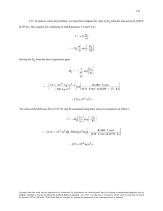
![5-35
5.28 In order to determine the temperature to which the diffusion couple must be heated so as to produce a
concentration of 3.0 wt% Ni at the 2.0-mm position, we must first utilize Equation 5.6b with time t being a constant.
That is
x2
D
= constant
Or
x1000
2
D1000
=
xT
2
DT
Now, solving for DT from this equation, yields
DT =
2 D1000
x1000
xT
2
and incorporating the temperature dependence of D1000 utilizing Equation (5.8), yields
DT =
xT
( 2)D0 exp −
Qd
RT
⎛
⎜
⎝
⎞
⎟
⎠
⎡
⎢
⎣
⎤
⎥
⎦
2
x1000
=
(2 mm)2 (2.7 × 10⁻⁴ m2 /s)exp − 236,000 J/mol
(8.31 J/mol - K)(1273 K)
⎛
⎜
⎝
⎞
⎟
⎠
⎡
⎢
⎣
⎢
⎤
⎥
⎦
⎥
(1 mm)2
= 2.21 x 10⁻¹³ m2/s
We now need to find the T at which D has this value. This is accomplished by rearranging Equation 5.9a and
solving for T as
T =
Qd
R (lnD0 − lnD)
= 236,000 J/mol
(8.31 J/mol - K)[ln (2.7 × 10⁻⁴ m2/s) − ln (2.21 × 10⁻¹³ m2/s)]
= 1357 K = 1084°C
Excerpts from this work may be reproduced by instructors for distribution on a not-for-profit basis for testing or instructional purposes only to
students enrolled in courses for which the textbook has been adopted. Any other reproduction or translation of this work beyond that permitted
by Sections 107 or 108 of the 1976 United States Copyright Act without the permission of the copyright owner is unlawful.](https://image.slidesharecdn.com/ecyluo1ys2qvoutji72q-signature-9b381c5777758ee4fe884904ded9f35d0b251da572c8ac51c821cb24bd095f1b-poli-141018125101-conversion-gate02/85/solution-for-Materials-Science-and-Engineering-7th-edition-by-William-D-Callister-Jr-189-320.jpg)

![5-39
= (3.5 × 10⁻³ m)2
(4)(172,800 s)(0.821)
= 2.16 × 10⁻¹¹ m2/s
Now, in order to determine the temperature at which D has the above value, we must employ Equation 5.9a;
solving this equation for T yields
T =
Qd
R (lnD0 − lnD)
From Table 5.2, D0 and Qd for the diffusion of C in FCC Fe are 2.3 x 10⁻⁵ m2/s and 148,000 J/mol, respectively.
Therefore
T = 148,000 J/mol
(8.31 J/mol - K) ln ([ 2.3 × 10⁻⁵ m2/s) - ln (2.16 × 10⁻¹¹ m2/s)]
= 1283 K = 1010°C
Excerpts from this work may be reproduced by instructors for distribution on a not-for-profit basis for testing or instructional purposes only to
students enrolled in courses for which the textbook has been adopted. Any other reproduction or translation of this work beyond that permitted
by Sections 107 or 108 of the 1976 United States Copyright Act without the permission of the copyright owner is unlawful.](https://image.slidesharecdn.com/ecyluo1ys2qvoutji72q-signature-9b381c5777758ee4fe884904ded9f35d0b251da572c8ac51c821cb24bd095f1b-poli-141018125101-conversion-gate02/85/solution-for-Materials-Science-and-Engineering-7th-edition-by-William-D-Callister-Jr-192-320.jpg)


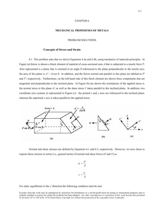
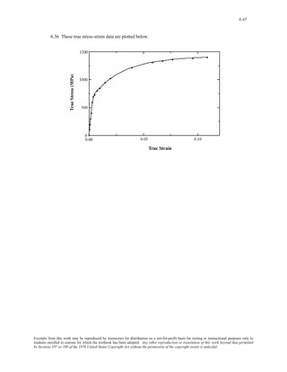
![6-2
ΣF x'
= 0
which means that
PÕ− P cos θ = 0
Or that
P' = P cos θ
Now it is possible to write an expression for the stress σ' in terms of P' and A' using the above expression and the
relationship between A and A' [Figure (a)]:
σ' = PÕ
AÕ
= P cosθ
A
cosθ
= P
A
cos2θ
However, it is the case that P/A = σ; and, after making this substitution into the above expression, we have
Equation 6.4a--that is
σ ' = σ cos2θ
Now, for static equilibrium in the y' direction, it is necessary that
ΣFyÕ= 0
= −VÕ+ Psinθ
Or
V ' = Psinθ
Excerpts from this work may be reproduced by instructors for distribution on a not-for-profit basis for testing or instructional purposes only to
students enrolled in courses for which the textbook has been adopted. Any other reproduction or translation of this work beyond that permitted
by Sections 107 or 108 of the 1976 United States Copyright Act without the permission of the copyright owner is unlawful.](https://image.slidesharecdn.com/ecyluo1ys2qvoutji72q-signature-9b381c5777758ee4fe884904ded9f35d0b251da572c8ac51c821cb24bd095f1b-poli-141018125101-conversion-gate02/85/solution-for-Materials-Science-and-Engineering-7th-edition-by-William-D-Callister-Jr-201-320.jpg)


![6-14
6.11 We are asked, using the equation given in the problem statement, to verify that the modulus of
elasticity values along [110] directions given in Table 3.3 for aluminum, copper, and iron are correct. The α, β, and
γ parameters in the equation correspond, respectively, to the cosines of the angles between the [110] direction and
[100], [010] and [001] directions. Since these angles are 45°, 45°, and 90°, the values of α, β, and γ are 0.707,
0.707, and 0, respectively. Thus, the given equation takes the form
1
E<110>
= 1
E<100>
− 3 1
E<100>
− 1
E<111>
⎛
⎜⎜
⎝
⎞
⎠
⎟⎟ [(0.707)2 (0.707)2 + (0.707)2 (0)2 + (0)2 (0.707)2]
= 1
E<100>
− (0.75) 1
E<100>
− 1
E<111>
⎛
⎜⎜
⎝
⎞
⎟⎟
⎠
Utilizing the values of E<100> and E<111> from Table 3.3 for Al
1
E<110>
= 1
63.7 GPa
− (0.75) 1
63.7 GPa
− 1
76.1 GPa
⎡
⎢
⎣
⎤
⎥
⎦
Which leads to, E<110> = 72.6 GPa, the value cited in the table.
For Cu,
1
E<110>
= 1
66.7 GPa
− (0.75) 1
66.7 GPa
− 1
191.1 GPa
⎡
⎢
⎣
⎤
⎥
⎦
Thus, E<110> = 130.3 GPa, which is also the value cited in the table.
Similarly, for Fe
1
E<110>
= 1
125.0 GPa
− (0.75) 1
125.0 GPa
− 1
272.7 GPa
⎡
⎢
⎣
⎤
⎥
⎦
And E<110> = 210.5 GPa, which is also the value given in the table.
Excerpts from this work may be reproduced by instructors for distribution on a not-for-profit basis for testing or instructional purposes only to
students enrolled in courses for which the textbook has been adopted. Any other reproduction or translation of this work beyond that permitted
by Sections 107 or 108 of the 1976 United States Copyright Act without the permission of the copyright owner is unlawful.](https://image.slidesharecdn.com/ecyluo1ys2qvoutji72q-signature-9b381c5777758ee4fe884904ded9f35d0b251da572c8ac51c821cb24bd095f1b-poli-141018125101-conversion-gate02/85/solution-for-Materials-Science-and-Engineering-7th-edition-by-William-D-Callister-Jr-213-320.jpg)


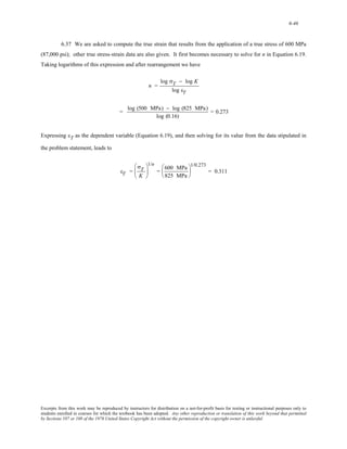


![6-50
6.41 This problem calls for us to compute the toughness (or energy to cause fracture). The easiest way to
do this is to integrate both elastic and plastic regions, and then add them together.
Toughness = ∫σ dε
0.007
∫ + Kεn d ε
= Eεd ε
0
0.60
∫
0.007
= Eε2
2
0.007
0
+ K
(n + 1)
ε(n+1)
0.60
0.007
= 103 x 109 N /m2
2
(0.007 )2 + 1520 x 106 N/ m2
(1.0 + 0.15)
[(0.60)1.15 − (0.007)1.15]
= 7.33 x 10⁸ J/m3 (1.07 x 105 in.-lbf/in.3)
Excerpts from this work may be reproduced by instructors for distribution on a not-for-profit basis for testing or instructional purposes only to
students enrolled in courses for which the textbook has been adopted. Any other reproduction or translation of this work beyond that permitted
by Sections 107 or 108 of the 1976 United States Copyright Act without the permission of the copyright owner is unlawful.](https://image.slidesharecdn.com/ecyluo1ys2qvoutji72q-signature-9b381c5777758ee4fe884904ded9f35d0b251da572c8ac51c821cb24bd095f1b-poli-141018125101-conversion-gate02/85/solution-for-Materials-Science-and-Engineering-7th-edition-by-William-D-Callister-Jr-248-320.jpg)
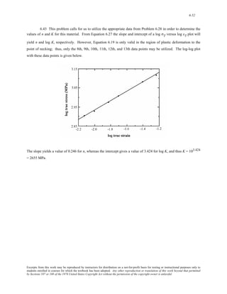
![6-51
6.42 This problem asks that we determine the value of εT for the onset of necking assuming that necking
begins when
d σT
d εT
= σT
Let us take the derivative of Equation 6.19, set it equal to σT, and then solve for εT from the resulting expression.
Thus
d[K (εT )n]
d εT
= Kn (εT )(n−1) = σT
However, from Equation 6.19, σT = K(εT)n, which, when substituted into the above expression, yields
Kn (εT )(n - 1) = K(εT )n
Now solving for εT from this equation leads to
εT = n
as the value of the true strain at the onset of necking.
Excerpts from this work may be reproduced by instructors for distribution on a not-for-profit basis for testing or instructional purposes only to
students enrolled in courses for which the textbook has been adopted. Any other reproduction or translation of this work beyond that permitted
by Sections 107 or 108 of the 1976 United States Copyright Act without the permission of the copyright owner is unlawful.](https://image.slidesharecdn.com/ecyluo1ys2qvoutji72q-signature-9b381c5777758ee4fe884904ded9f35d0b251da572c8ac51c821cb24bd095f1b-poli-141018125101-conversion-gate02/85/solution-for-Materials-Science-and-Engineering-7th-edition-by-William-D-Callister-Jr-249-320.jpg)

![6-56
6.47 This problem calls for estimations of Brinell and Rockwell hardnesses.
(a) For the brass specimen, the stress-strain behavior for which is shown in Figure 6.12, the tensile
strength is 450 MPa (65,000 psi). From Figure 6.19, the hardness for brass corresponding to this tensile strength is
about 125 HB or 70 HRB.
(b) The steel alloy (Figure 6.21) has a tensile strength of about 1970 MPa (285,000 psi) [Problem 6.24(d)].
This corresponds to a hardness of about 560 HB or ~55 HRC from the line (extended) for steels in Figure 6.19.
Excerpts from this work may be reproduced by instructors for distribution on a not-for-profit basis for testing or instructional purposes only to
students enrolled in courses for which the textbook has been adopted. Any other reproduction or translation of this work beyond that permitted
by Sections 107 or 108 of the 1976 United States Copyright Act without the permission of the copyright owner is unlawful.](https://image.slidesharecdn.com/ecyluo1ys2qvoutji72q-signature-9b381c5777758ee4fe884904ded9f35d0b251da572c8ac51c821cb24bd095f1b-poli-141018125101-conversion-gate02/85/solution-for-Materials-Science-and-Engineering-7th-edition-by-William-D-Callister-Jr-254-320.jpg)


![7-13
Slip in Single Crystals
7.11 We are asked to compute the Schmid factor for an FCC crystal oriented with its [120] direction
parallel to the loading axis. With this scheme, slip may occur on the (111) plane and in the [011 ] direction as noted
in the figure below.
The angle between the [120] and [011 ] directions, λ, may be determined using Equation 7.6
⎢
⎢
⎢
λ = cos−1 u1u2 + v1v2 + w1w2
( u1
2 + v1
2 + w1
2)u2
⎥
⎥
⎥
( 2 + v2
2 + w2
2)
⎡
⎣
⎤
⎦
where (for [120]) u1 = 1, v1 = 2, w1 = 0, and (for [011 ]) u2 = 0, v2 = 1, w2 = -1. Therefore, λ is equal to
⎢
⎢
⎢
λ = cos−1 (1)(0) + (2)(1) + (0)(−1)
⎥
⎥
⎥
[(1)2 + (2)2 + (0)2][(0)2 + (1)2 + (−1)2]
⎡
⎣
⎤
⎦
= cos−1 2
10
⎛
⎜⎜
⎝
⎞
⎠
⎟⎟ = 50.8°
Excerpts from this work may be reproduced by instructors for distribution on a not-for-profit basis for testing or instructional purposes only to
students enrolled in courses for which the textbook has been adopted. Any other reproduction or translation of this work beyond that permitted
by Sections 107 or 108 of the 1976 United States Copyright Act without the permission of the copyright owner is unlawful.](https://image.slidesharecdn.com/ecyluo1ys2qvoutji72q-signature-9b381c5777758ee4fe884904ded9f35d0b251da572c8ac51c821cb24bd095f1b-poli-141018125101-conversion-gate02/85/solution-for-Materials-Science-and-Engineering-7th-edition-by-William-D-Callister-Jr-278-320.jpg)
![7-14
Now, the angle φ is equal to the angle between the normal to the (111) plane (which is the [111] direction), and the
[120] direction. Again from Equation 7.6, and for u1 = 1, v1 = 1, w1 = 1, u2 = 1, v2 = 2, and w2 = 0, we have
⎢
⎢
⎢
φ = cos−1 (1)(1) + (1)(2) + (1)(0)
⎥
⎥
⎥
[(1)2 + (1)2 + (1)2][(1)2 + (2)2 + (0)2]
⎡
⎣
⎤
⎦
= cos−1 3
15
⎛
⎜⎜
⎝
⎞
⎠
⎟⎟ = 39.2°
Therefore, the Schmid factor is equal to
cos λ cos φ = cos(50.8°) cos(39.2°) = 2
10
⎛
⎜⎜
⎝
⎞
⎟⎟
⎠
3
15
⎛
⎜
⎝
⎞
⎠
⎟ = 0.490
Excerpts from this work may be reproduced by instructors for distribution on a not-for-profit basis for testing or instructional purposes only to
students enrolled in courses for which the textbook has been adopted. Any other reproduction or translation of this work beyond that permitted
by Sections 107 or 108 of the 1976 United States Copyright Act without the permission of the copyright owner is unlawful.](https://image.slidesharecdn.com/ecyluo1ys2qvoutji72q-signature-9b381c5777758ee4fe884904ded9f35d0b251da572c8ac51c821cb24bd095f1b-poli-141018125101-conversion-gate02/85/solution-for-Materials-Science-and-Engineering-7th-edition-by-William-D-Callister-Jr-279-320.jpg)

![7-16
7.13 We are asked to compute the critical resolved shear stress for Zn. As stipulated in the problem, φ =
65°, while possible values for λ are 30°, 48°, and 78°.
(a) Slip will occur along that direction for which (cos φ cos λ) is a maximum, or, in this case, for the
largest cos λ. Cosines for the possible λ values are given below.
cos(30°) = 0.87
cos(48°) = 0.67
cos(78°) = 0.21
Thus, the slip direction is at an angle of 30° with the tensile axis.
(b) From Equation 7.4, the critical resolved shear stress is just
τcrss = σ y (cos φ cos λ)max
= (2.5 MPa) [cos(65°) cos(30°)] = 0.90 MPa (130 psi)
Excerpts from this work may be reproduced by instructors for distribution on a not-for-profit basis for testing or instructional purposes only to
students enrolled in courses for which the textbook has been adopted. Any other reproduction or translation of this work beyond that permitted
by Sections 107 or 108 of the 1976 United States Copyright Act without the permission of the copyright owner is unlawful.](https://image.slidesharecdn.com/ecyluo1ys2qvoutji72q-signature-9b381c5777758ee4fe884904ded9f35d0b251da572c8ac51c821cb24bd095f1b-poli-141018125101-conversion-gate02/85/solution-for-Materials-Science-and-Engineering-7th-edition-by-William-D-Callister-Jr-281-320.jpg)
![7-17
7.14 This problem asks that we compute the critical resolved shear stress for nickel. In order to do this,
we must employ Equation 7.4, but first it is necessary to solve for the angles λ and φ which are shown in the sketch
below.
The angle λ is the angle between the tensile axis—i.e., along the [001] direction—and the slip direction—i.e.,
[1 01]. The angle λ may be determined using Equation 7.6 as
⎢
⎢
⎢
λ = cos−1 u1u2 + v1v2 + w1w2
( u1
2 + v1
2 + w1
2)u2
⎥
⎥
⎥
( 2 + v2
2 + w2
2)
⎡
⎣
⎤
⎦
where (for [001]) u1 = 0, v1 = 0, w1 = 1, and (for [1 01]) u2 = –1, v2 = 0, w2 = 1. Therefore, λ is equal to
⎢
⎢
⎢
λ = cos−1 (0)(−1) + (0)(0) + (1)(1)
⎥
⎥
⎥
[(0)2 + (0)2 + (1)2][(−1)2 + (0)2 + (1)2]
⎡
⎣
⎤
⎦
= cos−1 1
2
⎛
⎜⎜
⎝
⎞
⎠
⎟⎟ = 45°
Furthermore, φ is the angle between the tensile axis—the [001] direction—and the normal to the slip plane—i.e., the
(111) plane; for this case this normal is along a [111] direction. Therefore, again using Equation 7.6
Excerpts from this work may be reproduced by instructors for distribution on a not-for-profit basis for testing or instructional purposes only to
students enrolled in courses for which the textbook has been adopted. Any other reproduction or translation of this work beyond that permitted
by Sections 107 or 108 of the 1976 United States Copyright Act without the permission of the copyright owner is unlawful.](https://image.slidesharecdn.com/ecyluo1ys2qvoutji72q-signature-9b381c5777758ee4fe884904ded9f35d0b251da572c8ac51c821cb24bd095f1b-poli-141018125101-conversion-gate02/85/solution-for-Materials-Science-and-Engineering-7th-edition-by-William-D-Callister-Jr-282-320.jpg)
![7-18
⎢
⎢
⎢
φ = cos−1 (0)(1) + (0)(1) + (1)(1)
⎥
⎥
⎥
[(0)2 + (0)2 + (1)2][(1)2 + (1)2 + (1)2]
⎡
⎣
⎤
⎦
= cos−1 1
3
⎛
⎜⎜
⎝
⎞
⎠
⎟⎟ = 54.7°
And, finally, using Equation 7.4, the critical resolved shear stress is equal to
τcrss = σ y (cos φ cos λ)
= (13.9 MPa) [cos(54.7°) cos(45°)] = (13.9 MPa) 1
3
⎛
⎜⎜
⎝
⎞
⎟⎟
⎠
1
2
⎛
⎜⎜
⎝
⎞
⎠
⎟⎟ = 5.68 MPa (825 psi)
Excerpts from this work may be reproduced by instructors for distribution on a not-for-profit basis for testing or instructional purposes only to
students enrolled in courses for which the textbook has been adopted. Any other reproduction or translation of this work beyond that permitted
by Sections 107 or 108 of the 1976 United States Copyright Act without the permission of the copyright owner is unlawful.](https://image.slidesharecdn.com/ecyluo1ys2qvoutji72q-signature-9b381c5777758ee4fe884904ded9f35d0b251da572c8ac51c821cb24bd095f1b-poli-141018125101-conversion-gate02/85/solution-for-Materials-Science-and-Engineering-7th-edition-by-William-D-Callister-Jr-283-320.jpg)
![7-19
7.15 This problem asks that, for a metal that has the FCC crystal structure, we compute the applied
stress(s) that are required to cause slip to occur on a (111) plane in each of the [11 0 ], [101 ], and [01 1] directions.
In order to solve this problem it is necessary to employ Equation 7.4, but first we need to solve for the for λ and φ
angles for the three slip systems.
For each of these three slip systems, the φ will be the same—i.e., the angle between the direction of the
applied stress, [100] and the normal to the (111) plane, that is, the [111] direction. The angle φ may be determined
using Equation 7.6 as
⎢
⎢
⎢
φ = cos−1 u1u2 + v1v2 + w1w2
( u1
2 + v1
2 + w1
2)u2
⎥
⎥
⎥
( 2 + v2
2 + w2
2)
⎡
⎣
⎤
⎦
where (for [100]) u1 = 1, v1 = 0, w1 = 0, and (for [111]) u2 = 1, v2 = 1, w2 = 1. Therefore, φ is equal to
⎢
⎢
⎢
φ = cos−1 (1)(1) + (0)(1) + (0)(1)
⎥
⎥
⎥
[(1)2 + (0)2 + (0)2][(1)2 + (1)2 + (1)2]
⎡
⎣
⎤
⎦
= cos−1 1
3
⎛
⎜⎜
⎝
⎞
⎠
⎟⎟ = 54.7°
Let us now determine λ for the [11 0 ] slip direction. Again, using Equation 7.6 where u1 = 1, v1 = 0, w1 = 0 (for
[100]), and u2 = 1, v2 = –1, w2 = 0 (for [11 0]. Therefore, λ is determined as
⎢
⎢
⎢
λ[100]−[11 0] = cos−1 (1)(1) + (0)(−1) + (0)(0)
⎥
⎥
⎥
[(1)2 + (0)2 + (0)2][(1)2 + (−1)2 + (0)2]
⎡
⎣
⎤
⎦
= cos−1 1
2
⎛
⎜⎜
⎝
⎞
⎠
⎟⎟ = 45°
Now, we solve for the yield strength for this (111)–[11 0] slip system using Equation 7.4 as
σ y =
τcrss
(cosφ cos λ)
Excerpts from this work may be reproduced by instructors for distribution on a not-for-profit basis for testing or instructional purposes only to
students enrolled in courses for which the textbook has been adopted. Any other reproduction or translation of this work beyond that permitted
by Sections 107 or 108 of the 1976 United States Copyright Act without the permission of the copyright owner is unlawful.](https://image.slidesharecdn.com/ecyluo1ys2qvoutji72q-signature-9b381c5777758ee4fe884904ded9f35d0b251da572c8ac51c821cb24bd095f1b-poli-141018125101-conversion-gate02/85/solution-for-Materials-Science-and-Engineering-7th-edition-by-William-D-Callister-Jr-284-320.jpg)
![7-20
= 0.5 MPa
cos (54.7°) cos (45°)
= 0.5 MPa
(0.578) (0.707)
= 1.22 MPa
Now, we must determine the value of λ for the (111)–[101 ] slip system—that is, the angle between the
[100] and [101 ] directions. Again using Equation 7.6
⎢
⎢
⎢
λ[100]−[101 ] = cos−1 (1)(1) + (0)(0) + (0)(−1)
⎥
⎥
⎥
[(1)2 + (0)2 + (0)2][(1)2 + (0)2 + (−1)2]
⎡
⎣
⎤
⎦
= cos−1 1
2
⎛
⎜⎜
⎝
⎞
⎠
⎟⎟ = 45°
Thus, since the values of φ and λ for this (111)–[101 ] slip system are the same as for (111)–[11 0] , so also will σy
be the same—viz 1.22 MPa.
And, finally, for the (111)–[01 1] slip system, λ is computed using Equation 7.6 as follows:
⎢
⎢
⎢
λ[100]−[ 01 1] = cos−1 (1)(0) + (0)(−1) + (0)(1)
⎥
⎥
⎥
[(1)2 + (0)2 + (0)2][(0)2 + (−1)2 + (1)2]
⎡
⎣
⎤
⎦
= cos−1 (0) = 90°
Thus, from Equation 7.4, the yield strength for this slip system is
σ y =
τcrss
(cosφ cos λ)
= 0.5 MPa
cos (54.7°) cos (90°)
= 0.5 MPa
(0.578) (0)
= ∞
which means that slip will not occur on this (111)–[01 1] slip system.
Excerpts from this work may be reproduced by instructors for distribution on a not-for-profit basis for testing or instructional purposes only to
students enrolled in courses for which the textbook has been adopted. Any other reproduction or translation of this work beyond that permitted
by Sections 107 or 108 of the 1976 United States Copyright Act without the permission of the copyright owner is unlawful.](https://image.slidesharecdn.com/ecyluo1ys2qvoutji72q-signature-9b381c5777758ee4fe884904ded9f35d0b251da572c8ac51c821cb24bd095f1b-poli-141018125101-conversion-gate02/85/solution-for-Materials-Science-and-Engineering-7th-edition-by-William-D-Callister-Jr-285-320.jpg)
![7-21
7.16 (a) This part of the problem asks, for a BCC metal, that we compute the resolved shear stress in the
[11 1] direction on each of the (110), (011), and (101 ) planes. In order to solve this problem it is necessary to
employ Equation 7.2, which means that we first need to solve for the for angles λ and φ for the three slip systems.
For each of these three slip systems, the λ will be the same—i.e., the angle between the direction of the
applied stress, [100] and the slip direction, [11 1]. This angle λ may be determined using Equation 7.6
⎢
⎢
⎢
λ = cos−1 u1u2 + v1v2 + w1w2
( u1
2 + v1
2 + w1
2)u2
⎥
⎥
⎥
( 2 + v2
2 + w2
2)
⎡
⎣
⎤
⎦
where (for [100]) u1 = 1, v1 = 0, w1 = 0, and (for [11 1]) u2 = 1, v2 = –1, w2 = 1. Therefore, λ is determined as
⎢
⎢
⎢
λ = cos−1 (1)(1) + (0)(−1) + (0)(1)
⎥
⎥
⎥
[(1)2 + (0)2 + (0)2][(1)2 + (−1)2 + (1)2]
⎡
⎣
⎤
⎦
= cos−1 1
3
⎛
⎜⎜
⎝
⎞
⎠
⎟⎟ = 54.7°
Let us now determine φ for the angle between the direction of the applied tensile stress—i.e., the [100] direction—
and the normal to the (110) slip plane—i.e., the [110] direction. Again, using Equation 7.6 where u1 = 1, v1 = 0, w1
= 0 (for [100]), and u2 = 1, v2 = 1, w2 = 0 (for [110]), φ is equal to
⎢
⎢
⎢
φ[100]−[110] = cos−1 (1)(1) + (0)(1) + (0)(0)
⎥
⎥
⎥
[(1)2 + (0)2 + (0)2][(1)2 + (1)2 + (0)2]
⎡
⎣
⎤
⎦
= cos−1 1
2
⎛
⎜⎜
⎝
⎞
⎠
⎟⎟ = 45°
Now, using Equation 7.2
τR = σ cosφ cos λ
we solve for the resolved shear stress for this slip system as
Excerpts from this work may be reproduced by instructors for distribution on a not-for-profit basis for testing or instructional purposes only to
students enrolled in courses for which the textbook has been adopted. Any other reproduction or translation of this work beyond that permitted
by Sections 107 or 108 of the 1976 United States Copyright Act without the permission of the copyright owner is unlawful.](https://image.slidesharecdn.com/ecyluo1ys2qvoutji72q-signature-9b381c5777758ee4fe884904ded9f35d0b251da572c8ac51c821cb24bd095f1b-poli-141018125101-conversion-gate02/85/solution-for-Materials-Science-and-Engineering-7th-edition-by-William-D-Callister-Jr-286-320.jpg)
![7-22
τR(110)−[11 1] = (4.0 MPa) [cos (45°) cos (54.7°)] = (4.0 MPa) (0.707)(0.578) = 1.63 MPa
Now, we must determine the value of φ for the (011)–[11 1] slip system—that is, the angle between the
direction of the applied stress, [100], and the normal to the (011) plane—i.e., the [011] direction. Again using
Equation 7.6
⎢
⎢
⎢
λ[100]−[ 011] = cos−1 (1)(0) + (0)(1) + (0)(1)
⎥
⎥
⎥
[(1)2 + (0)2 + (0)2][(0)2 + (1)2 + (1)2]
⎡
⎣
⎤
⎦
= cos−1 (0) = 90°
Thus, the resolved shear stress for this (011)–[11 1] slip system is
τR(011)−[11 1] = = (4.0 MPa) [cos (90°) cos (54.7°)] = (4.0 MPa) (0)(0.578) = 0 MPa
And, finally, it is necessary to determine the value of φ for the (101 )–[11 1] slip system —that is, the
angle between the direction of the applied stress, [100], and the normal to the (101 ) plane—i.e., the [101 ]
direction. Again using Equation 7.6
⎢
⎢
⎢
λ[100]−[101 ] = cos−1 (1)(1) + (0)(0) + (0)(−1)
⎥
⎥
⎥
[(1)2 + (0)2 + (0)2][(1)2 + (0)2 + (−1)2]
⎡
⎣
⎤
⎦
= cos−1 1
2
⎛
⎜⎜
⎝
⎞
⎠
⎟⎟ = 45°
Here, as with the (110)–[11 1] slip system above, the value of φ is 45°, which again leads to
τR(101 )−[11 1] = (4.0 MPa) [cos (45°) cos (54.7°)] = (4.0 MPa) (0.707)(0.578) = 1.63 MPa
(b) The most favored slip system(s) is (are) the one(s) that has (have) the largest τR value. Both (110)–
[11 1] and (101 ) −[11 1] slip systems are most favored since they have the same τR (1.63 MPa), which is greater
than the τR value for (011) −[11 1] (viz., 0 MPa).
Excerpts from this work may be reproduced by instructors for distribution on a not-for-profit basis for testing or instructional purposes only to
students enrolled in courses for which the textbook has been adopted. Any other reproduction or translation of this work beyond that permitted
by Sections 107 or 108 of the 1976 United States Copyright Act without the permission of the copyright owner is unlawful.](https://image.slidesharecdn.com/ecyluo1ys2qvoutji72q-signature-9b381c5777758ee4fe884904ded9f35d0b251da572c8ac51c821cb24bd095f1b-poli-141018125101-conversion-gate02/85/solution-for-Materials-Science-and-Engineering-7th-edition-by-William-D-Callister-Jr-287-320.jpg)
![7-23
7.17 This problem asks for us to determine the tensile stress at which a BCC metal yields when the stress
is applied along a [121] direction such that slip occurs on a (101) plane and in a [1 11] direction; the critical
resolved shear stress for this metal is 2.4 MPa. To solve this problem we use Equation 7.4; however it is first
necessary to determine the values of φ and λ. These determinations are possible using Equation 7.6. Now, λ is the
angle between [121] and [1 11] directions. Therefore, relative to Equation 7.6 let us take u1 = 1, v1 = 2, and w1 =
1, as well as u2 = –1, v2 = 1, and w2 = 1. This leads to
⎢
⎢
⎢
λ = cos−1 u1u2 + v1v2 + w1w2
( u1
2 + v1
2 + w1
2)u2
⎥
⎥
⎥
( 2 + v2
2 + w2
2)
⎡
⎣
⎤
⎦
= cos−1 (1)(−1) + (2)(1) + (1)(1)
[(1)2 + (2)2 + (1)2][(−1)2 + (1)2 + (1)2]
⎧
⎪
⎨
⎪
⎩
⎫
⎪
⎬
⎪
⎭
= cos−1 2
18
⎛
⎜⎜
⎝
⎞
⎠
⎟⎟ = 61.9°
Now for the determination of φ, the normal to the (101) slip plane is the [101] direction. Again using Equation 7.6,
where we now take u1 = 1, v1 = 2, w1 = 1 (for [121]), and u2 = 1, v2 = 0, w2 = 1 (for [101]). Thus,
φ = cos−1 (1)(1) + (2)(0) + (1)(1)
[(1)2 + (2)2 + (1)2][(1)2 + (0)2 + (1)2]
⎧
⎪
⎨
⎪
⎩
⎫
⎪
⎬
⎪
⎭
= cos−1 2
12
⎛
⎜⎜
⎝
⎞
⎠
⎟⎟ = 54.7°
It is now possible to compute the yield stress (using Equation 7.4) as
σ y =
τcrss
cosφ cos λ
= 2.4 MPa
2
12
⎛
⎜⎜
⎝
⎞
⎟⎟
⎠
2
18
⎛
⎜⎜
⎝
⎞
⎟⎟
⎠
= 8.82 MPa
Excerpts from this work may be reproduced by instructors for distribution on a not-for-profit basis for testing or instructional purposes only to
students enrolled in courses for which the textbook has been adopted. Any other reproduction or translation of this work beyond that permitted
by Sections 107 or 108 of the 1976 United States Copyright Act without the permission of the copyright owner is unlawful.](https://image.slidesharecdn.com/ecyluo1ys2qvoutji72q-signature-9b381c5777758ee4fe884904ded9f35d0b251da572c8ac51c821cb24bd095f1b-poli-141018125101-conversion-gate02/85/solution-for-Materials-Science-and-Engineering-7th-edition-by-William-D-Callister-Jr-288-320.jpg)


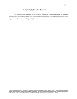
![7-29
7.23 (a) Perhaps the easiest way to solve for σ0 and ky in Equation 7.7 is to pick two values each of σy
and d-1/2 from Figure 7.15, and then solve two simultaneous equations, which may be set up. For example
d-1/2 (mm) -1/2 σy (MPa)
4 75
12 175
The two equations are thus
75 = σ0 + 4k y
175 = σ0 + 12k y
Solution of these equations yield the values of
k y = 12.5 MPa (mm)1/2 [1810 psi (mm)1/2]
σ0 = 25 MPa (3630 psi)
(b) When d = 2.0 x 10⁻³ mm, d-1/2 = 22.4 mm-1/2, and, using Equation 7.7,
σ y = σ0 + k yd-1/2
⎡ 1/2
⎢⎣
= (25 MPa) + 12.5 MPa (mm)
⎤
⎥⎦ (22.4 mm-1/2) = 305 MPa (44,200 psi)
Excerpts from this work may be reproduced by instructors for distribution on a not-for-profit basis for testing or instructional purposes only to
students enrolled in courses for which the textbook has been adopted. Any other reproduction or translation of this work beyond that permitted
by Sections 107 or 108 of the 1976 United States Copyright Act without the permission of the copyright owner is unlawful.](https://image.slidesharecdn.com/ecyluo1ys2qvoutji72q-signature-9b381c5777758ee4fe884904ded9f35d0b251da572c8ac51c821cb24bd095f1b-poli-141018125101-conversion-gate02/85/solution-for-Materials-Science-and-Engineering-7th-edition-by-William-D-Callister-Jr-294-320.jpg)
![7-30
7.24 We are asked to determine the grain diameter for an iron which will give a yield strength of 310 MPa
(45,000 psi). The best way to solve this problem is to first establish two simultaneous expressions of Equation 7.7,
solve for σ0 and ky, and finally determine the value of d when σy = 310 MPa. The data pertaining to this problem
may be tabulated as follows:
σy d (mm) d-1/2 (mm)-1/2
230 MPa 1 x 10⁻² 10.0
275 MPa 6 x 10⁻³ 12.91
The two equations thus become
230 MPa = σ0 + (10.0) k y
275 MPa = σ0 + (12.91) k y
Which yield the values, σ0 = 75.4 MPa and ky = 15.46 MPa(mm)1/2. At a yield strength of 310 MPa
310 MPa = 75.4 MPa + [15.46 MPa (mm)1/2]d-1/2
or d-1/2 = 15.17 (mm)-1/2, which gives d = 4.34 x 10⁻³ mm.
Excerpts from this work may be reproduced by instructors for distribution on a not-for-profit basis for testing or instructional purposes only to
students enrolled in courses for which the textbook has been adopted. Any other reproduction or translation of this work beyond that permitted
by Sections 107 or 108 of the 1976 United States Copyright Act without the permission of the copyright owner is unlawful.](https://image.slidesharecdn.com/ecyluo1ys2qvoutji72q-signature-9b381c5777758ee4fe884904ded9f35d0b251da572c8ac51c821cb24bd095f1b-poli-141018125101-conversion-gate02/85/solution-for-Materials-Science-and-Engineering-7th-edition-by-William-D-Callister-Jr-295-320.jpg)


![7-37
7.31 (a) We want to compute the ductility of a brass that has a yield strength of 345 MPa (50,000 psi). In
order to solve this problem, it is necessary to consult Figures 7.19(a) and (c). From Figure 7.19(a), a yield strength
of 345 MPa for brass corresponds to 20%CW. A brass that has been cold-worked 20% will have a ductility of
about 24%EL [Figure 7.19(c)].
(b) This portion of the problem asks for the Brinell hardness of a 1040 steel having a yield strength of 620
MPa (90,000 psi). From Figure 7.19(a), a yield strength of 620 MPa for a 1040 steel corresponds to about 5%CW.
A 1040 steel that has been cold worked 5% will have a tensile strength of about 750 MPa [Figure 7.19(b)]. Finally,
using Equation 6.20a
HB = TS(MPa)
3.45
= 750 MPa
3.45
= 217
Excerpts from this work may be reproduced by instructors for distribution on a not-for-profit basis for testing or instructional purposes only to
students enrolled in courses for which the textbook has been adopted. Any other reproduction or translation of this work beyond that permitted
by Sections 107 or 108 of the 1976 United States Copyright Act without the permission of the copyright owner is unlawful.](https://image.slidesharecdn.com/ecyluo1ys2qvoutji72q-signature-9b381c5777758ee4fe884904ded9f35d0b251da572c8ac51c821cb24bd095f1b-poli-141018125101-conversion-gate02/85/solution-for-Materials-Science-and-Engineering-7th-edition-by-William-D-Callister-Jr-302-320.jpg)

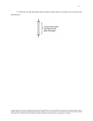


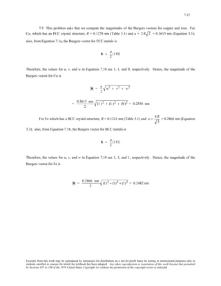

![7-13
Slip in Single Crystals
7.11 We are asked to compute the Schmid factor for an FCC crystal oriented with its [120] direction
parallel to the loading axis. With this scheme, slip may occur on the (111) plane and in the [011 ] direction as noted
in the figure below.
The angle between the [120] and [011 ] directions, λ, may be determined using Equation 7.6
⎢
⎢
⎢
λ = cos−1 u1u2 + v1v2 + w1w2
( u1
2 + v1
2 + w1
2)u2
⎥
⎥
⎥
( 2 + v2
2 + w2
2)
⎡
⎣
⎤
⎦
where (for [120]) u1 = 1, v1 = 2, w1 = 0, and (for [011 ]) u2 = 0, v2 = 1, w2 = -1. Therefore, λ is equal to
⎢
⎢
⎢
λ = cos−1 (1)(0) + (2)(1) + (0)(−1)
⎥
⎥
⎥
[(1)2 + (2)2 + (0)2][(0)2 + (1)2 + (−1)2]
⎡
⎣
⎤
⎦
= cos−1 2
10
⎛
⎜⎜
⎝
⎞
⎠
⎟⎟ = 50.8°
Excerpts from this work may be reproduced by instructors for distribution on a not-for-profit basis for testing or instructional purposes only to
students enrolled in courses for which the textbook has been adopted. Any other reproduction or translation of this work beyond that permitted
by Sections 107 or 108 of the 1976 United States Copyright Act without the permission of the copyright owner is unlawful.](https://image.slidesharecdn.com/ecyluo1ys2qvoutji72q-signature-9b381c5777758ee4fe884904ded9f35d0b251da572c8ac51c821cb24bd095f1b-poli-141018125101-conversion-gate02/85/solution-for-Materials-Science-and-Engineering-7th-edition-by-William-D-Callister-Jr-316-320.jpg)
![7-14
Now, the angle φ is equal to the angle between the normal to the (111) plane (which is the [111] direction), and the
[120] direction. Again from Equation 7.6, and for u1 = 1, v1 = 1, w1 = 1, u2 = 1, v2 = 2, and w2 = 0, we have
⎢
⎢
⎢
φ = cos−1 (1)(1) + (1)(2) + (1)(0)
⎥
⎥
⎥
[(1)2 + (1)2 + (1)2][(1)2 + (2)2 + (0)2]
⎡
⎣
⎤
⎦
= cos−1 3
15
⎛
⎜⎜
⎝
⎞
⎠
⎟⎟ = 39.2°
Therefore, the Schmid factor is equal to
cos λ cos φ = cos(50.8°) cos(39.2°) = 2
10
⎛
⎜⎜
⎝
⎞
⎟⎟
⎠
3
15
⎛
⎜
⎝
⎞
⎠
⎟ = 0.490
Excerpts from this work may be reproduced by instructors for distribution on a not-for-profit basis for testing or instructional purposes only to
students enrolled in courses for which the textbook has been adopted. Any other reproduction or translation of this work beyond that permitted
by Sections 107 or 108 of the 1976 United States Copyright Act without the permission of the copyright owner is unlawful.](https://image.slidesharecdn.com/ecyluo1ys2qvoutji72q-signature-9b381c5777758ee4fe884904ded9f35d0b251da572c8ac51c821cb24bd095f1b-poli-141018125101-conversion-gate02/85/solution-for-Materials-Science-and-Engineering-7th-edition-by-William-D-Callister-Jr-317-320.jpg)

![7-16
7.13 We are asked to compute the critical resolved shear stress for Zn. As stipulated in the problem, φ =
65°, while possible values for λ are 30°, 48°, and 78°.
(a) Slip will occur along that direction for which (cos φ cos λ) is a maximum, or, in this case, for the
largest cos λ. Cosines for the possible λ values are given below.
cos(30°) = 0.87
cos(48°) = 0.67
cos(78°) = 0.21
Thus, the slip direction is at an angle of 30° with the tensile axis.
(b) From Equation 7.4, the critical resolved shear stress is just
τcrss = σ y (cos φ cos λ)max
= (2.5 MPa) [cos(65°) cos(30°)] = 0.90 MPa (130 psi)
Excerpts from this work may be reproduced by instructors for distribution on a not-for-profit basis for testing or instructional purposes only to
students enrolled in courses for which the textbook has been adopted. Any other reproduction or translation of this work beyond that permitted
by Sections 107 or 108 of the 1976 United States Copyright Act without the permission of the copyright owner is unlawful.](https://image.slidesharecdn.com/ecyluo1ys2qvoutji72q-signature-9b381c5777758ee4fe884904ded9f35d0b251da572c8ac51c821cb24bd095f1b-poli-141018125101-conversion-gate02/85/solution-for-Materials-Science-and-Engineering-7th-edition-by-William-D-Callister-Jr-319-320.jpg)
![7-17
7.14 This problem asks that we compute the critical resolved shear stress for nickel. In order to do this,
we must employ Equation 7.4, but first it is necessary to solve for the angles λ and φ which are shown in the sketch
below.
The angle λ is the angle between the tensile axis—i.e., along the [001] direction—and the slip direction—i.e.,
[1 01]. The angle λ may be determined using Equation 7.6 as
⎢
⎢
⎢
λ = cos−1 u1u2 + v1v2 + w1w2
( u1
2 + v1
2 + w1
2)u2
⎥
⎥
⎥
( 2 + v2
2 + w2
2)
⎡
⎣
⎤
⎦
where (for [001]) u1 = 0, v1 = 0, w1 = 1, and (for [1 01]) u2 = –1, v2 = 0, w2 = 1. Therefore, λ is equal to
⎢
⎢
⎢
λ = cos−1 (0)(−1) + (0)(0) + (1)(1)
⎥
⎥
⎥
[(0)2 + (0)2 + (1)2][(−1)2 + (0)2 + (1)2]
⎡
⎣
⎤
⎦
= cos−1 1
2
⎛
⎜⎜
⎝
⎞
⎠
⎟⎟ = 45°
Furthermore, φ is the angle between the tensile axis—the [001] direction—and the normal to the slip plane—i.e., the
(111) plane; for this case this normal is along a [111] direction. Therefore, again using Equation 7.6
Excerpts from this work may be reproduced by instructors for distribution on a not-for-profit basis for testing or instructional purposes only to
students enrolled in courses for which the textbook has been adopted. Any other reproduction or translation of this work beyond that permitted
by Sections 107 or 108 of the 1976 United States Copyright Act without the permission of the copyright owner is unlawful.](https://image.slidesharecdn.com/ecyluo1ys2qvoutji72q-signature-9b381c5777758ee4fe884904ded9f35d0b251da572c8ac51c821cb24bd095f1b-poli-141018125101-conversion-gate02/85/solution-for-Materials-Science-and-Engineering-7th-edition-by-William-D-Callister-Jr-320-320.jpg)
![7-18
⎢
⎢
⎢
φ = cos−1 (0)(1) + (0)(1) + (1)(1)
⎥
⎥
⎥
[(0)2 + (0)2 + (1)2][(1)2 + (1)2 + (1)2]
⎡
⎣
⎤
⎦
= cos−1 1
3
⎛
⎜⎜
⎝
⎞
⎠
⎟⎟ = 54.7°
And, finally, using Equation 7.4, the critical resolved shear stress is equal to
τcrss = σ y (cos φ cos λ)
= (13.9 MPa) [cos(54.7°) cos(45°)] = (13.9 MPa) 1
3
⎛
⎜⎜
⎝
⎞
⎟⎟
⎠
1
2
⎛
⎜⎜
⎝
⎞
⎠
⎟⎟ = 5.68 MPa (825 psi)
Excerpts from this work may be reproduced by instructors for distribution on a not-for-profit basis for testing or instructional purposes only to
students enrolled in courses for which the textbook has been adopted. Any other reproduction or translation of this work beyond that permitted
by Sections 107 or 108 of the 1976 United States Copyright Act without the permission of the copyright owner is unlawful.](https://image.slidesharecdn.com/ecyluo1ys2qvoutji72q-signature-9b381c5777758ee4fe884904ded9f35d0b251da572c8ac51c821cb24bd095f1b-poli-141018125101-conversion-gate02/85/solution-for-Materials-Science-and-Engineering-7th-edition-by-William-D-Callister-Jr-321-320.jpg)
![7-19
7.15 This problem asks that, for a metal that has the FCC crystal structure, we compute the applied
stress(s) that are required to cause slip to occur on a (111) plane in each of the [11 0 ], [101 ], and [01 1] directions.
In order to solve this problem it is necessary to employ Equation 7.4, but first we need to solve for the for λ and φ
angles for the three slip systems.
For each of these three slip systems, the φ will be the same—i.e., the angle between the direction of the
applied stress, [100] and the normal to the (111) plane, that is, the [111] direction. The angle φ may be determined
using Equation 7.6 as
⎢
⎢
⎢
φ = cos−1 u1u2 + v1v2 + w1w2
( u1
2 + v1
2 + w1
2)u2
⎥
⎥
⎥
( 2 + v2
2 + w2
2)
⎡
⎣
⎤
⎦
where (for [100]) u1 = 1, v1 = 0, w1 = 0, and (for [111]) u2 = 1, v2 = 1, w2 = 1. Therefore, φ is equal to
⎢
⎢
⎢
φ = cos−1 (1)(1) + (0)(1) + (0)(1)
⎥
⎥
⎥
[(1)2 + (0)2 + (0)2][(1)2 + (1)2 + (1)2]
⎡
⎣
⎤
⎦
= cos−1 1
3
⎛
⎜⎜
⎝
⎞
⎠
⎟⎟ = 54.7°
Let us now determine λ for the [11 0 ] slip direction. Again, using Equation 7.6 where u1 = 1, v1 = 0, w1 = 0 (for
[100]), and u2 = 1, v2 = –1, w2 = 0 (for [11 0]. Therefore, λ is determined as
⎢
⎢
⎢
λ[100]−[11 0] = cos−1 (1)(1) + (0)(−1) + (0)(0)
⎥
⎥
⎥
[(1)2 + (0)2 + (0)2][(1)2 + (−1)2 + (0)2]
⎡
⎣
⎤
⎦
= cos−1 1
2
⎛
⎜⎜
⎝
⎞
⎠
⎟⎟ = 45°
Now, we solve for the yield strength for this (111)–[11 0] slip system using Equation 7.4 as
σ y =
τcrss
(cosφ cos λ)
Excerpts from this work may be reproduced by instructors for distribution on a not-for-profit basis for testing or instructional purposes only to
students enrolled in courses for which the textbook has been adopted. Any other reproduction or translation of this work beyond that permitted
by Sections 107 or 108 of the 1976 United States Copyright Act without the permission of the copyright owner is unlawful.](https://image.slidesharecdn.com/ecyluo1ys2qvoutji72q-signature-9b381c5777758ee4fe884904ded9f35d0b251da572c8ac51c821cb24bd095f1b-poli-141018125101-conversion-gate02/85/solution-for-Materials-Science-and-Engineering-7th-edition-by-William-D-Callister-Jr-322-320.jpg)
![7-20
= 0.5 MPa
cos (54.7°) cos (45°)
= 0.5 MPa
(0.578) (0.707)
= 1.22 MPa
Now, we must determine the value of λ for the (111)–[101 ] slip system—that is, the angle between the
[100] and [101 ] directions. Again using Equation 7.6
⎢
⎢
⎢
λ[100]−[101 ] = cos−1 (1)(1) + (0)(0) + (0)(−1)
⎥
⎥
⎥
[(1)2 + (0)2 + (0)2][(1)2 + (0)2 + (−1)2]
⎡
⎣
⎤
⎦
= cos−1 1
2
⎛
⎜⎜
⎝
⎞
⎠
⎟⎟ = 45°
Thus, since the values of φ and λ for this (111)–[101 ] slip system are the same as for (111)–[11 0] , so also will σy
be the same—viz 1.22 MPa.
And, finally, for the (111)–[01 1] slip system, λ is computed using Equation 7.6 as follows:
⎢
⎢
⎢
λ[100]−[ 01 1] = cos−1 (1)(0) + (0)(−1) + (0)(1)
⎥
⎥
⎥
[(1)2 + (0)2 + (0)2][(0)2 + (−1)2 + (1)2]
⎡
⎣
⎤
⎦
= cos−1 (0) = 90°
Thus, from Equation 7.4, the yield strength for this slip system is
σ y =
τcrss
(cosφ cos λ)
= 0.5 MPa
cos (54.7°) cos (90°)
= 0.5 MPa
(0.578) (0)
= ∞
which means that slip will not occur on this (111)–[01 1] slip system.
Excerpts from this work may be reproduced by instructors for distribution on a not-for-profit basis for testing or instructional purposes only to
students enrolled in courses for which the textbook has been adopted. Any other reproduction or translation of this work beyond that permitted
by Sections 107 or 108 of the 1976 United States Copyright Act without the permission of the copyright owner is unlawful.](https://image.slidesharecdn.com/ecyluo1ys2qvoutji72q-signature-9b381c5777758ee4fe884904ded9f35d0b251da572c8ac51c821cb24bd095f1b-poli-141018125101-conversion-gate02/85/solution-for-Materials-Science-and-Engineering-7th-edition-by-William-D-Callister-Jr-323-320.jpg)
![7-21
7.16 (a) This part of the problem asks, for a BCC metal, that we compute the resolved shear stress in the
[11 1] direction on each of the (110), (011), and (101 ) planes. In order to solve this problem it is necessary to
employ Equation 7.2, which means that we first need to solve for the for angles λ and φ for the three slip systems.
For each of these three slip systems, the λ will be the same—i.e., the angle between the direction of the
applied stress, [100] and the slip direction, [11 1]. This angle λ may be determined using Equation 7.6
⎢
⎢
⎢
λ = cos−1 u1u2 + v1v2 + w1w2
( u1
2 + v1
2 + w1
2)u2
⎥
⎥
⎥
( 2 + v2
2 + w2
2)
⎡
⎣
⎤
⎦
where (for [100]) u1 = 1, v1 = 0, w1 = 0, and (for [11 1]) u2 = 1, v2 = –1, w2 = 1. Therefore, λ is determined as
⎢
⎢
⎢
λ = cos−1 (1)(1) + (0)(−1) + (0)(1)
⎥
⎥
⎥
[(1)2 + (0)2 + (0)2][(1)2 + (−1)2 + (1)2]
⎡
⎣
⎤
⎦
= cos−1 1
3
⎛
⎜⎜
⎝
⎞
⎠
⎟⎟ = 54.7°
Let us now determine φ for the angle between the direction of the applied tensile stress—i.e., the [100] direction—
and the normal to the (110) slip plane—i.e., the [110] direction. Again, using Equation 7.6 where u1 = 1, v1 = 0, w1
= 0 (for [100]), and u2 = 1, v2 = 1, w2 = 0 (for [110]), φ is equal to
⎢
⎢
⎢
φ[100]−[110] = cos−1 (1)(1) + (0)(1) + (0)(0)
⎥
⎥
⎥
[(1)2 + (0)2 + (0)2][(1)2 + (1)2 + (0)2]
⎡
⎣
⎤
⎦
= cos−1 1
2
⎛
⎜⎜
⎝
⎞
⎠
⎟⎟ = 45°
Now, using Equation 7.2
τR = σ cosφ cos λ
we solve for the resolved shear stress for this slip system as
Excerpts from this work may be reproduced by instructors for distribution on a not-for-profit basis for testing or instructional purposes only to
students enrolled in courses for which the textbook has been adopted. Any other reproduction or translation of this work beyond that permitted
by Sections 107 or 108 of the 1976 United States Copyright Act without the permission of the copyright owner is unlawful.](https://image.slidesharecdn.com/ecyluo1ys2qvoutji72q-signature-9b381c5777758ee4fe884904ded9f35d0b251da572c8ac51c821cb24bd095f1b-poli-141018125101-conversion-gate02/85/solution-for-Materials-Science-and-Engineering-7th-edition-by-William-D-Callister-Jr-324-320.jpg)
![7-22
τR(110)−[11 1] = (4.0 MPa) [cos (45°) cos (54.7°)] = (4.0 MPa) (0.707)(0.578) = 1.63 MPa
Now, we must determine the value of φ for the (011)–[11 1] slip system—that is, the angle between the
direction of the applied stress, [100], and the normal to the (011) plane—i.e., the [011] direction. Again using
Equation 7.6
⎢
⎢
⎢
λ[100]−[ 011] = cos−1 (1)(0) + (0)(1) + (0)(1)
⎥
⎥
⎥
[(1)2 + (0)2 + (0)2][(0)2 + (1)2 + (1)2]
⎡
⎣
⎤
⎦
= cos−1 (0) = 90°
Thus, the resolved shear stress for this (011)–[11 1] slip system is
τR(011)−[11 1] = = (4.0 MPa) [cos (90°) cos (54.7°)] = (4.0 MPa) (0)(0.578) = 0 MPa
And, finally, it is necessary to determine the value of φ for the (101 )–[11 1] slip system —that is, the
angle between the direction of the applied stress, [100], and the normal to the (101 ) plane—i.e., the [101 ]
direction. Again using Equation 7.6
⎢
⎢
⎢
λ[100]−[101 ] = cos−1 (1)(1) + (0)(0) + (0)(−1)
⎥
⎥
⎥
[(1)2 + (0)2 + (0)2][(1)2 + (0)2 + (−1)2]
⎡
⎣
⎤
⎦
= cos−1 1
2
⎛
⎜⎜
⎝
⎞
⎠
⎟⎟ = 45°
Here, as with the (110)–[11 1] slip system above, the value of φ is 45°, which again leads to
τR(101 )−[11 1] = (4.0 MPa) [cos (45°) cos (54.7°)] = (4.0 MPa) (0.707)(0.578) = 1.63 MPa
(b) The most favored slip system(s) is (are) the one(s) that has (have) the largest τR value. Both (110)–
[11 1] and (101 ) −[11 1] slip systems are most favored since they have the same τR (1.63 MPa), which is greater
than the τR value for (011) −[11 1] (viz., 0 MPa).
Excerpts from this work may be reproduced by instructors for distribution on a not-for-profit basis for testing or instructional purposes only to
students enrolled in courses for which the textbook has been adopted. Any other reproduction or translation of this work beyond that permitted
by Sections 107 or 108 of the 1976 United States Copyright Act without the permission of the copyright owner is unlawful.](https://image.slidesharecdn.com/ecyluo1ys2qvoutji72q-signature-9b381c5777758ee4fe884904ded9f35d0b251da572c8ac51c821cb24bd095f1b-poli-141018125101-conversion-gate02/85/solution-for-Materials-Science-and-Engineering-7th-edition-by-William-D-Callister-Jr-325-320.jpg)
![7-23
7.17 This problem asks for us to determine the tensile stress at which a BCC metal yields when the stress
is applied along a [121] direction such that slip occurs on a (101) plane and in a [1 11] direction; the critical
resolved shear stress for this metal is 2.4 MPa. To solve this problem we use Equation 7.4; however it is first
necessary to determine the values of φ and λ. These determinations are possible using Equation 7.6. Now, λ is the
angle between [121] and [1 11] directions. Therefore, relative to Equation 7.6 let us take u1 = 1, v1 = 2, and w1 =
1, as well as u2 = –1, v2 = 1, and w2 = 1. This leads to
⎢
⎢
⎢
λ = cos−1 u1u2 + v1v2 + w1w2
( u1
2 + v1
2 + w1
2)u2
⎥
⎥
⎥
( 2 + v2
2 + w2
2)
⎡
⎣
⎤
⎦
= cos−1 (1)(−1) + (2)(1) + (1)(1)
[(1)2 + (2)2 + (1)2][(−1)2 + (1)2 + (1)2]
⎧
⎪
⎨
⎪
⎩
⎫
⎪
⎬
⎪
⎭
= cos−1 2
18
⎛
⎜⎜
⎝
⎞
⎠
⎟⎟ = 61.9°
Now for the determination of φ, the normal to the (101) slip plane is the [101] direction. Again using Equation 7.6,
where we now take u1 = 1, v1 = 2, w1 = 1 (for [121]), and u2 = 1, v2 = 0, w2 = 1 (for [101]). Thus,
φ = cos−1 (1)(1) + (2)(0) + (1)(1)
[(1)2 + (2)2 + (1)2][(1)2 + (0)2 + (1)2]
⎧
⎪
⎨
⎪
⎩
⎫
⎪
⎬
⎪
⎭
= cos−1 2
12
⎛
⎜⎜
⎝
⎞
⎠
⎟⎟ = 54.7°
It is now possible to compute the yield stress (using Equation 7.4) as
σ y =
τcrss
cosφ cos λ
= 2.4 MPa
2
12
⎛
⎜⎜
⎝
⎞
⎟⎟
⎠
2
18
⎛
⎜⎜
⎝
⎞
⎟⎟
⎠
= 8.82 MPa
Excerpts from this work may be reproduced by instructors for distribution on a not-for-profit basis for testing or instructional purposes only to
students enrolled in courses for which the textbook has been adopted. Any other reproduction or translation of this work beyond that permitted
by Sections 107 or 108 of the 1976 United States Copyright Act without the permission of the copyright owner is unlawful.](https://image.slidesharecdn.com/ecyluo1ys2qvoutji72q-signature-9b381c5777758ee4fe884904ded9f35d0b251da572c8ac51c821cb24bd095f1b-poli-141018125101-conversion-gate02/85/solution-for-Materials-Science-and-Engineering-7th-edition-by-William-D-Callister-Jr-326-320.jpg)


![7-29
7.23 (a) Perhaps the easiest way to solve for σ0 and ky in Equation 7.7 is to pick two values each of σy
and d-1/2 from Figure 7.15, and then solve two simultaneous equations, which may be set up. For example
d-1/2 (mm) -1/2 σy (MPa)
4 75
12 175
The two equations are thus
75 = σ0 + 4k y
175 = σ0 + 12k y
Solution of these equations yield the values of
k y = 12.5 MPa (mm)1/2 [1810 psi (mm)1/2]
σ0 = 25 MPa (3630 psi)
(b) When d = 2.0 x 10⁻³ mm, d-1/2 = 22.4 mm-1/2, and, using Equation 7.7,
σ y = σ0 + k yd-1/2
⎡ 1/2
⎢⎣
= (25 MPa) + 12.5 MPa (mm)
⎤
⎥⎦ (22.4 mm-1/2) = 305 MPa (44,200 psi)
Excerpts from this work may be reproduced by instructors for distribution on a not-for-profit basis for testing or instructional purposes only to
students enrolled in courses for which the textbook has been adopted. Any other reproduction or translation of this work beyond that permitted
by Sections 107 or 108 of the 1976 United States Copyright Act without the permission of the copyright owner is unlawful.](https://image.slidesharecdn.com/ecyluo1ys2qvoutji72q-signature-9b381c5777758ee4fe884904ded9f35d0b251da572c8ac51c821cb24bd095f1b-poli-141018125101-conversion-gate02/85/solution-for-Materials-Science-and-Engineering-7th-edition-by-William-D-Callister-Jr-332-320.jpg)
![7-30
7.24 We are asked to determine the grain diameter for an iron which will give a yield strength of 310 MPa
(45,000 psi). The best way to solve this problem is to first establish two simultaneous expressions of Equation 7.7,
solve for σ0 and ky, and finally determine the value of d when σy = 310 MPa. The data pertaining to this problem
may be tabulated as follows:
σy d (mm) d-1/2 (mm)-1/2
230 MPa 1 x 10⁻² 10.0
275 MPa 6 x 10⁻³ 12.91
The two equations thus become
230 MPa = σ0 + (10.0) k y
275 MPa = σ0 + (12.91) k y
Which yield the values, σ0 = 75.4 MPa and ky = 15.46 MPa(mm)1/2. At a yield strength of 310 MPa
310 MPa = 75.4 MPa + [15.46 MPa (mm)1/2]d-1/2
or d-1/2 = 15.17 (mm)-1/2, which gives d = 4.34 x 10⁻³ mm.
Excerpts from this work may be reproduced by instructors for distribution on a not-for-profit basis for testing or instructional purposes only to
students enrolled in courses for which the textbook has been adopted. Any other reproduction or translation of this work beyond that permitted
by Sections 107 or 108 of the 1976 United States Copyright Act without the permission of the copyright owner is unlawful.](https://image.slidesharecdn.com/ecyluo1ys2qvoutji72q-signature-9b381c5777758ee4fe884904ded9f35d0b251da572c8ac51c821cb24bd095f1b-poli-141018125101-conversion-gate02/85/solution-for-Materials-Science-and-Engineering-7th-edition-by-William-D-Callister-Jr-333-320.jpg)


![7-37
7.31 (a) We want to compute the ductility of a brass that has a yield strength of 345 MPa (50,000 psi). In
order to solve this problem, it is necessary to consult Figures 7.19(a) and (c). From Figure 7.19(a), a yield strength
of 345 MPa for brass corresponds to 20%CW. A brass that has been cold-worked 20% will have a ductility of
about 24%EL [Figure 7.19(c)].
(b) This portion of the problem asks for the Brinell hardness of a 1040 steel having a yield strength of 620
MPa (90,000 psi). From Figure 7.19(a), a yield strength of 620 MPa for a 1040 steel corresponds to about 5%CW.
A 1040 steel that has been cold worked 5% will have a tensile strength of about 750 MPa [Figure 7.19(b)]. Finally,
using Equation 6.20a
HB = TS(MPa)
3.45
= 750 MPa
3.45
= 217
Excerpts from this work may be reproduced by instructors for distribution on a not-for-profit basis for testing or instructional purposes only to
students enrolled in courses for which the textbook has been adopted. Any other reproduction or translation of this work beyond that permitted
by Sections 107 or 108 of the 1976 United States Copyright Act without the permission of the copyright owner is unlawful.](https://image.slidesharecdn.com/ecyluo1ys2qvoutji72q-signature-9b381c5777758ee4fe884904ded9f35d0b251da572c8ac51c821cb24bd095f1b-poli-141018125101-conversion-gate02/85/solution-for-Materials-Science-and-Engineering-7th-edition-by-William-D-Callister-Jr-340-320.jpg)
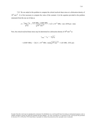


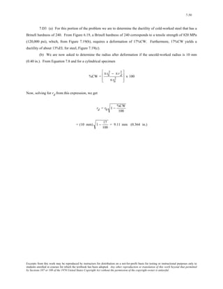

![7-52
7.D5 This problem calls for us to explain the procedure by which a cylindrical rod of 1040 steel may be
deformed so as to produce a given final diameter (8.9 mm), as well as a specific minimum tensile strength (825
MPa) and minimum ductility (12%EL). First let us calculate the percent cold work and attendant tensile strength
and ductility if the drawing is carried out without interruption. From Equation 7.8
%CW =
π
d0
2
⎛
⎜
⎝
⎞
⎟
⎠
2
− π
dd
2
⎛
⎜
⎝
⎞
⎟
⎠
2
π
d0
2
⎛
⎜
⎝
⎞
⎟
⎠
2 x 100
=
π 11.4 mm
2
⎛
⎜
⎝
⎞
⎟
⎠
2
− π 8.9 mm
2
⎛
⎜
⎝
⎞
⎟
⎠
2
π 11.4 mm
2
⎛
⎜
⎝
⎞
⎟
⎠
2 x 100 = 40%CW
At 40%CW, the steel will have a tensile strength on the order of 900 MPa (130,000 psi) [Figure 7.19(b)], which is
adequate; however, the ductility will be less than 9%EL [Figure 7.19(c)], which is insufficient.
Instead of performing the drawing in a single operation, let us initially draw some fraction of the total
deformation, then anneal to recrystallize, and, finally, cold-work the material a second time in order to achieve the
final diameter, tensile strength, and ductility.
Reference to Figure 7.19(b) indicates that 17%CW is necessary to yield a tensile strength of 825 MPa
(122,000 psi). Similarly, a maximum of 19%CW is possible for 12%EL [Figure 7.19(c)]. The average of these
extremes is 18%CW. If the final diameter after the first drawing is d '
0 , then
18%CW =
π
d0 ' 2
⎛
⎜
⎜
⎝
⎞
⎟
⎟
⎠
2
− π 8.9 mm
2
⎛
⎜
⎝
⎞
⎟
⎠
2
π
d0 '
2
⎛
⎜
⎜
⎝
⎞
⎟
⎟
⎠
2 x 100
And, solving for , yields d0 ' d0 '
= 8.9 mm
1 − 18%CW
100
= 9.83 mm (0.387 in.)
Excerpts from this work may be reproduced by instructors for distribution on a not-for-profit basis for testing or instructional purposes only to
students enrolled in courses for which the textbook has been adopted. Any other reproduction or translation of this work beyond that permitted
by Sections 107 or 108 of the 1976 United States Copyright Act without the permission of the copyright owner is unlawful.](https://image.slidesharecdn.com/ecyluo1ys2qvoutji72q-signature-9b381c5777758ee4fe884904ded9f35d0b251da572c8ac51c821cb24bd095f1b-poli-141018125101-conversion-gate02/85/solution-for-Materials-Science-and-Engineering-7th-edition-by-William-D-Callister-Jr-355-320.jpg)
![7-53
7.D6 Let us first calculate the percent cold work and attendant yield strength and ductility if the drawing is
carried out without interruption. From Equation 7.8
%CW =
π
d0
2
⎛
⎜
⎝
⎞
⎟
⎠
2
− π
dd
2
⎛
⎜
⎝
⎞
⎟
⎠
2
π
d0
2
⎛
⎜
⎝
⎞
⎟
⎠
2 x 100
=
π 10.2 mm
2
⎛
⎜
⎝
⎞
⎟
⎠
2
− π 7.6 mm
2
⎛
⎜
⎝
⎞
⎟
⎠
2
π 10.2 mm
2
⎛
⎜
⎝
⎞
⎟
⎠
2 x 100 = 44.5%CW
At 44.5%CW, the brass will have a yield strength on the order of 420 MPa (61,000 psi), Figure 7.19(a), which is
adequate; however, the ductility will be about 5%EL, Figure 7.19(c), which is insufficient.
Instead of performing the drawing in a single operation, let us initially draw some fraction of the total
deformation, then anneal to recrystallize, and, finally, cold work the material a second time in order to achieve the
final diameter, yield strength, and ductility.
Reference to Figure 7.19(a) indicates that 27.5%CW is necessary to give a yield strength of 380 MPa.
Similarly, a maximum of 27.5%CW is possible for 15%EL [Figure 7.19(c)]. Thus, to achieve both the specified
yield strength and ductility, the brass must be deformed to 27.5 %CW. If the final diameter after the first drawing is
, then, using Equation 7.8 d0 '
27.5%CW =
π
d0 ' 2
⎛
⎜
⎜
⎝
⎞
⎟
⎟
⎠
2
− π 7.6 mm
2
⎛
⎜
⎝
⎞
⎟
⎠
2
π
d0 '
2
⎛
⎜
⎜
⎝
⎞
⎟
⎟
⎠
2 x 100
And, solving for yields d0 '
d0 '
= 7.6 mm
1 − 27.5%CW
100
= 8.93 mm (0.351 in.)
Excerpts from this work may be reproduced by instructors for distribution on a not-for-profit basis for testing or instructional purposes only to
students enrolled in courses for which the textbook has been adopted. Any other reproduction or translation of this work beyond that permitted
by Sections 107 or 108 of the 1976 United States Copyright Act without the permission of the copyright owner is unlawful.](https://image.slidesharecdn.com/ecyluo1ys2qvoutji72q-signature-9b381c5777758ee4fe884904ded9f35d0b251da572c8ac51c821cb24bd095f1b-poli-141018125101-conversion-gate02/85/solution-for-Materials-Science-and-Engineering-7th-edition-by-William-D-Callister-Jr-356-320.jpg)


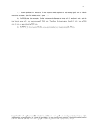
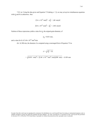


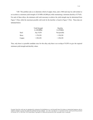
![7-52
7.D5 This problem calls for us to explain the procedure by which a cylindrical rod of 1040 steel may be
deformed so as to produce a given final diameter (8.9 mm), as well as a specific minimum tensile strength (825
MPa) and minimum ductility (12%EL). First let us calculate the percent cold work and attendant tensile strength
and ductility if the drawing is carried out without interruption. From Equation 7.8
%CW =
π
d0
2
⎛
⎜
⎝
⎞
⎟
⎠
2
− π
dd
2
⎛
⎜
⎝
⎞
⎟
⎠
2
π
d0
2
⎛
⎜
⎝
⎞
⎟
⎠
2 x 100
=
π 11.4 mm
2
⎛
⎜
⎝
⎞
⎟
⎠
2
− π 8.9 mm
2
⎛
⎜
⎝
⎞
⎟
⎠
2
π 11.4 mm
2
⎛
⎜
⎝
⎞
⎟
⎠
2 x 100 = 40%CW
At 40%CW, the steel will have a tensile strength on the order of 900 MPa (130,000 psi) [Figure 7.19(b)], which is
adequate; however, the ductility will be less than 9%EL [Figure 7.19(c)], which is insufficient.
Instead of performing the drawing in a single operation, let us initially draw some fraction of the total
deformation, then anneal to recrystallize, and, finally, cold-work the material a second time in order to achieve the
final diameter, tensile strength, and ductility.
Reference to Figure 7.19(b) indicates that 17%CW is necessary to yield a tensile strength of 825 MPa
(122,000 psi). Similarly, a maximum of 19%CW is possible for 12%EL [Figure 7.19(c)]. The average of these
extremes is 18%CW. If the final diameter after the first drawing is d '
0 , then
18%CW =
π
d0 ' 2
⎛
⎜
⎜
⎝
⎞
⎟
⎟
⎠
2
− π 8.9 mm
2
⎛
⎜
⎝
⎞
⎟
⎠
2
π
d0 '
2
⎛
⎜
⎜
⎝
⎞
⎟
⎟
⎠
2 x 100
And, solving for , yields d0 ' d0 '
= 8.9 mm
1 − 18%CW
100
= 9.83 mm (0.387 in.)
Excerpts from this work may be reproduced by instructors for distribution on a not-for-profit basis for testing or instructional purposes only to
students enrolled in courses for which the textbook has been adopted. Any other reproduction or translation of this work beyond that permitted
by Sections 107 or 108 of the 1976 United States Copyright Act without the permission of the copyright owner is unlawful.](https://image.slidesharecdn.com/ecyluo1ys2qvoutji72q-signature-9b381c5777758ee4fe884904ded9f35d0b251da572c8ac51c821cb24bd095f1b-poli-141018125101-conversion-gate02/85/solution-for-Materials-Science-and-Engineering-7th-edition-by-William-D-Callister-Jr-371-320.jpg)
![7-53
7.D6 Let us first calculate the percent cold work and attendant yield strength and ductility if the drawing is
carried out without interruption. From Equation 7.8
%CW =
π
d0
2
⎛
⎜
⎝
⎞
⎟
⎠
2
− π
dd
2
⎛
⎜
⎝
⎞
⎟
⎠
2
π
d0
2
⎛
⎜
⎝
⎞
⎟
⎠
2 x 100
=
π 10.2 mm
2
⎛
⎜
⎝
⎞
⎟
⎠
2
− π 7.6 mm
2
⎛
⎜
⎝
⎞
⎟
⎠
2
π 10.2 mm
2
⎛
⎜
⎝
⎞
⎟
⎠
2 x 100 = 44.5%CW
At 44.5%CW, the brass will have a yield strength on the order of 420 MPa (61,000 psi), Figure 7.19(a), which is
adequate; however, the ductility will be about 5%EL, Figure 7.19(c), which is insufficient.
Instead of performing the drawing in a single operation, let us initially draw some fraction of the total
deformation, then anneal to recrystallize, and, finally, cold work the material a second time in order to achieve the
final diameter, yield strength, and ductility.
Reference to Figure 7.19(a) indicates that 27.5%CW is necessary to give a yield strength of 380 MPa.
Similarly, a maximum of 27.5%CW is possible for 15%EL [Figure 7.19(c)]. Thus, to achieve both the specified
yield strength and ductility, the brass must be deformed to 27.5 %CW. If the final diameter after the first drawing is
, then, using Equation 7.8 d0 '
27.5%CW =
π
d0 ' 2
⎛
⎜
⎜
⎝
⎞
⎟
⎟
⎠
2
− π 7.6 mm
2
⎛
⎜
⎝
⎞
⎟
⎠
2
π
d0 '
2
⎛
⎜
⎜
⎝
⎞
⎟
⎟
⎠
2 x 100
And, solving for yields d0 '
d0 '
= 7.6 mm
1 − 27.5%CW
100
= 8.93 mm (0.351 in.)
Excerpts from this work may be reproduced by instructors for distribution on a not-for-profit basis for testing or instructional purposes only to
students enrolled in courses for which the textbook has been adopted. Any other reproduction or translation of this work beyond that permitted
by Sections 107 or 108 of the 1976 United States Copyright Act without the permission of the copyright owner is unlawful.](https://image.slidesharecdn.com/ecyluo1ys2qvoutji72q-signature-9b381c5777758ee4fe884904ded9f35d0b251da572c8ac51c821cb24bd095f1b-poli-141018125101-conversion-gate02/85/solution-for-Materials-Science-and-Engineering-7th-edition-by-William-D-Callister-Jr-372-320.jpg)
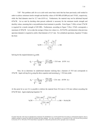

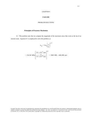


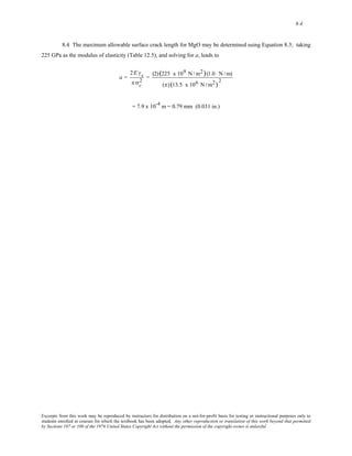


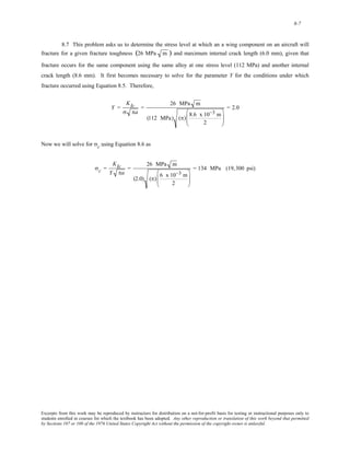
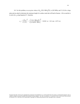


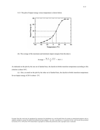


![8-18
8.18 (a) The fatigue data for this alloy are plotted below.
(b) As indicated by one set of dashed lines on the plot, the fatigue strength at 4 x 10⁶ cycles [log (4 x 10⁶)
= 6.6] is about 100 MPa.
(c) As noted by the other set of dashed lines, the fatigue life for 120 MPa is about 6 x 10⁵ cycles (i.e., the
log of the lifetime is about 5.8).
Excerpts from this work may be reproduced by instructors for distribution on a not-for-profit basis for testing or instructional purposes only to
students enrolled in courses for which the textbook has been adopted. Any other reproduction or translation of this work beyond that permitted
by Sections 107 or 108 of the 1976 United States Copyright Act without the permission of the copyright owner is unlawful.](https://image.slidesharecdn.com/ecyluo1ys2qvoutji72q-signature-9b381c5777758ee4fe884904ded9f35d0b251da572c8ac51c821cb24bd095f1b-poli-141018125101-conversion-gate02/85/solution-for-Materials-Science-and-Engineering-7th-edition-by-William-D-Callister-Jr-392-320.jpg)
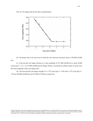


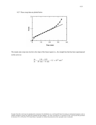
![8-29
Stress and Temperature Effects
8.28 This problem asks that we determine the total elongation of a low carbon-nickel alloy that is exposed
to a tensile stress of 70 MPa (10,000 psi) at 427°C for 10,000 h; the instantaneous and primary creep elongations
are 1.3 mm (0.05 in.).
From the 427°C line in Figure 8.31, the steady state creep rate Ýε s is about 4.7 x 10⁻⁷ h-1 at 70 MPa. The
steady state creep strain, εs, therefore, is just the product of Ýε s and time as
εs = Ýε s x (time)
= (4.7 x 10⁻⁷ h-1)(10,000 h) = 4.7 x10⁻³
Strain and elongation are related as in Equation 6.2; solving for the steady state elongation, Δls, leads to
Δls = l0 εs = (1015 mm) (4.7 x 10⁻³) = 4.8 mm (0.19 in.)
Finally, the total elongation is just the sum of this Δls and the total of both instantaneous and primary creep
elongations [i.e., 1.3 mm (0.05 in.)]. Therefore, the total elongation is 4.8 mm + 1.3 mm = 6.1 mm (0.24 in.).
Excerpts from this work may be reproduced by instructors for distribution on a not-for-profit basis for testing or instructional purposes only to
students enrolled in courses for which the textbook has been adopted. Any other reproduction or translation of this work beyond that permitted
by Sections 107 or 108 of the 1976 United States Copyright Act without the permission of the copyright owner is unlawful.](https://image.slidesharecdn.com/ecyluo1ys2qvoutji72q-signature-9b381c5777758ee4fe884904ded9f35d0b251da572c8ac51c821cb24bd095f1b-poli-141018125101-conversion-gate02/85/solution-for-Materials-Science-and-Engineering-7th-edition-by-William-D-Callister-Jr-403-320.jpg)
![8-30
8.29 We are asked to determine the tensile load necessary to elongate a 635 mm long low carbon-nickel
alloy specimen 6.44 mm after 5,000 h at 538°C. It is first necessary to calculate the steady state creep rate so that
we may utilize Figure 8.31 in order to determine the tensile stress. The steady state elongation, Δls, is just the
difference between the total elongation and the sum of the instantaneous and primary creep elongations; that is,
Δls = 6.44 mm − 1.8 mm = 4.64 mm (0.18 in.)
Now the steady state creep rate, εÝ s is just
εÝ s =
Δε
Δ t
=
Δ ls
l0
Δ t
=
4.64 mm
635 mm
5,000 h
= 1.46 x 10⁻⁶ h-1
Employing the 538°C line in Figure 8.31, a steady state creep rate of 1.46 x 10⁻⁶ h-1 corresponds to a stress σ of
about 40 MPa (5,800 psi) [since log (1.46 x 10⁻⁶) = -5.836]. From this we may compute the tensile load using
Equation 6.1 as
F = σA0 = σπ
d0
2
⎛
⎜
⎝
⎞
⎟
⎠
2
= (40 x 106 N/m2)(π) 19.0 x 10⁻³ m
2
⎛
⎜⎜
⎝
⎞
⎟⎟
⎠
2
= 11,300 N (2560 lbf )
Excerpts from this work may be reproduced by instructors for distribution on a not-for-profit basis for testing or instructional purposes only to
students enrolled in courses for which the textbook has been adopted. Any other reproduction or translation of this work beyond that permitted
by Sections 107 or 108 of the 1976 United States Copyright Act without the permission of the copyright owner is unlawful.](https://image.slidesharecdn.com/ecyluo1ys2qvoutji72q-signature-9b381c5777758ee4fe884904ded9f35d0b251da572c8ac51c821cb24bd095f1b-poli-141018125101-conversion-gate02/85/solution-for-Materials-Science-and-Engineering-7th-edition-by-William-D-Callister-Jr-404-320.jpg)


![8-34
8.33 (a) We are asked to estimate the activation energy for creep for the low carbon-nickel alloy having
the steady-state creep behavior shown in Figure 8.31, using data taken at σ = 55 MPa (8000 psi) and temperatures
of 427°C and 538°C. Since σ is a constant, Equation 8.20 takes the form
εÝ s = K2σnexp −
Qc
RT
⎛
⎜
⎝
⎞
⎠
⎟ = K2 '
exp −
Qc
RT
⎛
⎜
⎝
⎞
⎟
⎠
K2 '
where is now a constant. (Note: the exponent n has about the same value at these two temperatures per
Problem 8.32.) Taking natural logarithms of the above expression
ln Ý ε s = ln K2 '
−
Qc
RT
For the case in which we have creep data at two temperatures (denoted as T1 and T2) and their corresponding
steady-state creep rates ( Ýε s1
and Ýε s2
), it is possible to set up two simultaneous equations of the form as above, with
two unknowns, namely and Qc. Solving for Qc yields K2 '
Qc = −
R ln εÝ s 1
− ln εÝ s 2
⎛
⎝
⎜ ⎟
⎞
⎠
1
T1
− 1
T2
⎡
⎢
⎣
⎢
⎤
⎥
⎦
⎥
Let us choose T1 as 427°C (700 K) and T2 as 538°C (811 K); then from Figure 8.31, at σ = 55 MPa, Ýε s1
= 10-7 h-1
and Ýε s2
= 8 x 10⁻⁶ h-1. Substitution of these values into the above equation leads to
Qc = −
(8.31 J /mol - K)[ln (10−7 ) − ln (8 x 10⁻⁶)]
1
700 K
− 1
811 K
⎡
⎢⎣
⎤
⎥⎦
= 186,200 J/mol
(b) We are now asked to estimate Ýε s at 649°C (922 K). It is first necessary to determine the value of ,
which is accomplished using the first expression above, the value of Qc, and one value each of
K2 '
Ýε s and T (say Ýε s1
and T1). Thus,
Excerpts from this work may be reproduced by instructors for distribution on a not-for-profit basis for testing or instructional purposes only to
students enrolled in courses for which the textbook has been adopted. Any other reproduction or translation of this work beyond that permitted
by Sections 107 or 108 of the 1976 United States Copyright Act without the permission of the copyright owner is unlawful.](https://image.slidesharecdn.com/ecyluo1ys2qvoutji72q-signature-9b381c5777758ee4fe884904ded9f35d0b251da572c8ac51c821cb24bd095f1b-poli-141018125101-conversion-gate02/85/solution-for-Materials-Science-and-Engineering-7th-edition-by-William-D-Callister-Jr-408-320.jpg)


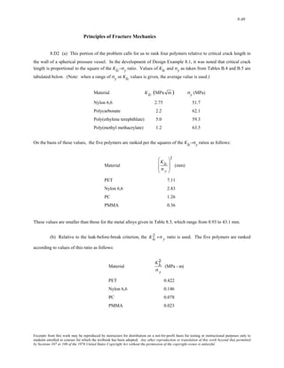

![8-42
Data Extrapolation Methods
8.D3 This problem asks that we compute the maximum allowable stress level to give a rupture lifetime of
20 days for an S-590 iron component at 923 K. It is first necessary to compute the value of the Larson-Miller
parameter as follows:
T (20 + log tr ) = (923 K){20 + log [(20 days)(24 h/day)]}
= 20.9 x 10³
From the curve in Figure 8.32, this value of the Larson-Miller parameter corresponds to a stress level of about 280
MPa (40,000 psi).
Excerpts from this work may be reproduced by instructors for distribution on a not-for-profit basis for testing or instructional purposes only to
students enrolled in courses for which the textbook has been adopted. Any other reproduction or translation of this work beyond that permitted
by Sections 107 or 108 of the 1976 United States Copyright Act without the permission of the copyright owner is unlawful.](https://image.slidesharecdn.com/ecyluo1ys2qvoutji72q-signature-9b381c5777758ee4fe884904ded9f35d0b251da572c8ac51c821cb24bd095f1b-poli-141018125101-conversion-gate02/85/solution-for-Materials-Science-and-Engineering-7th-edition-by-William-D-Callister-Jr-416-320.jpg)
![8-43
8.D4 We are asked in this problem to calculate the temperature at which the rupture lifetime is 200 h when
an S-590 iron component is subjected to a stress of 55 MPa (8000 psi). From the curve shown in Figure 8.32, at 55
MPa, the value of the Larson-Miller parameter is 26.7 x 10³ (K-h). Thus,
26.7 x 10³ (K - h) = T (20 + log tr )
= T [20 + log(200 h)]
Or, solving for T yields T = 1197 K (924°C).
Excerpts from this work may be reproduced by instructors for distribution on a not-for-profit basis for testing or instructional purposes only to
students enrolled in courses for which the textbook has been adopted. Any other reproduction or translation of this work beyond that permitted
by Sections 107 or 108 of the 1976 United States Copyright Act without the permission of the copyright owner is unlawful.](https://image.slidesharecdn.com/ecyluo1ys2qvoutji72q-signature-9b381c5777758ee4fe884904ded9f35d0b251da572c8ac51c821cb24bd095f1b-poli-141018125101-conversion-gate02/85/solution-for-Materials-Science-and-Engineering-7th-edition-by-William-D-Callister-Jr-417-320.jpg)

![8-45
8.D6 We are asked in this problem to calculate the stress levels at which the rupture lifetime will be 1 year
and 15 years when an 18-8 Mo stainless steel component is subjected to a temperature of 650°C (923 K). It first
becomes necessary to calculate the value of the Larson-Miller parameter for each time. The values of tr
corresponding to 1 and 15 years are 8.76 x 10³ h and 1.31 x 10⁵ h, respectively. Hence, for a lifetime of 1 year
T (20 + log tr ) = 923[20 + log (8.76 x 10³)]= 22.10 x 10³
And for tr = 15 years
T (20 + log tr ) = 923[20 + log (1.31 x 10⁵)]= 23.18 x 10³
Using the curve shown in Figure 8.35, the stress values corresponding to the one- and fifteen-year lifetimes
are approximately 110 MPa (16,000 psi) and 80 MPa (11,600 psi), respectively.
Excerpts from this work may be reproduced by instructors for distribution on a not-for-profit basis for testing or instructional purposes only to
students enrolled in courses for which the textbook has been adopted. Any other reproduction or translation of this work beyond that permitted
by Sections 107 or 108 of the 1976 United States Copyright Act without the permission of the copyright owner is unlawful.](https://image.slidesharecdn.com/ecyluo1ys2qvoutji72q-signature-9b381c5777758ee4fe884904ded9f35d0b251da572c8ac51c821cb24bd095f1b-poli-141018125101-conversion-gate02/85/solution-for-Materials-Science-and-Engineering-7th-edition-by-William-D-Callister-Jr-419-320.jpg)


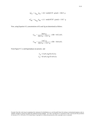


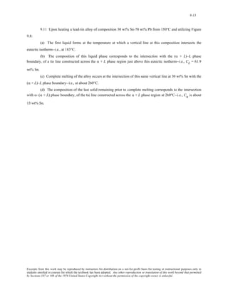


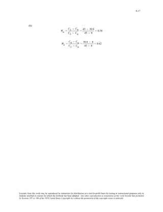


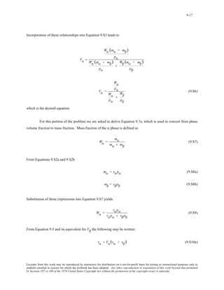


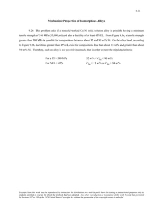

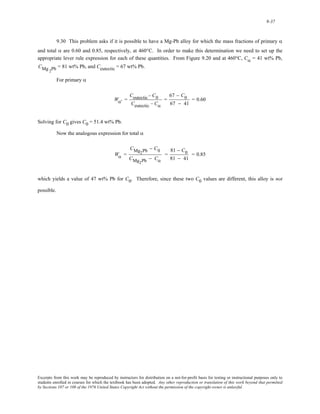


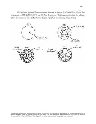
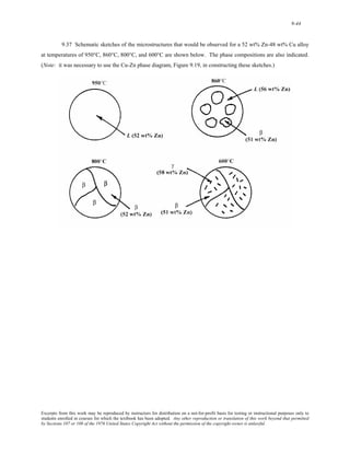

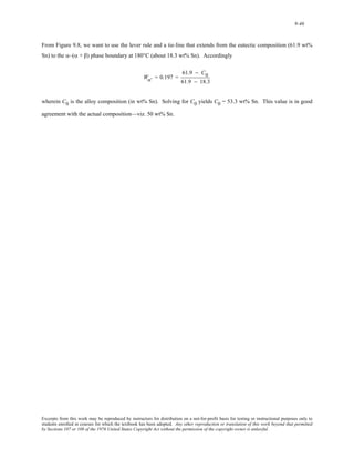
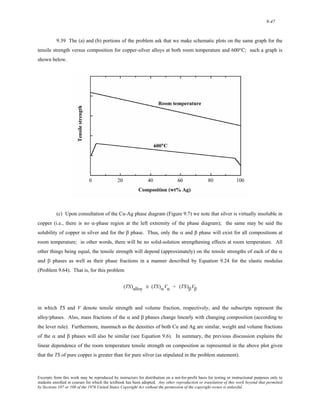
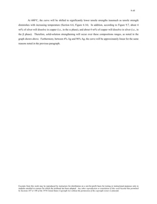


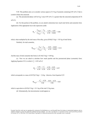


![10-9
n* = (1.52 x 1041 nuclei /m3)exp − 1.44 x10⁻¹⁸ J
(1.38 x 10⁻²³ J /atom− K) (1455 K − 300 K)
⎡
⎢
⎣
⎢
⎤
⎥
⎦
⎥
= 88 stable nuclei
(b) Relative to critical radius, r* for 300 K supercooling is slightly smaller that for 200 K (1.16 nm versus
1.74 nm). [From Problem 10.4, the value of r* at the homogeneous nucleation temperature (319 K) was 1.09 nm.]
More significant, however, are the values of n* at these two degrees of supercooling, which are dramatically
different—8.60 x 10-41 stable nuclei at ΔT = 200 K, versus 88 stable nuclei at ΔT = 300 K!
Excerpts from this work may be reproduced by instructors for distribution on a not-for-profit basis for testing or instructional purposes only to
students enrolled in courses for which the textbook has been adopted. Any other reproduction or translation of this work beyond that permitted
by Sections 107 or 108 of the 1976 United States Copyright Act without the permission of the copyright owner is unlawful.](https://image.slidesharecdn.com/ecyluo1ys2qvoutji72q-signature-9b381c5777758ee4fe884904ded9f35d0b251da572c8ac51c821cb24bd095f1b-poli-141018125101-conversion-gate02/85/solution-for-Materials-Science-and-Engineering-7th-edition-by-William-D-Callister-Jr-506-320.jpg)


![10-17
Solving these two expressions simultaneously for n and k yields n = 5.286 and k = 1.239 x 10⁻¹¹.
Now it becomes necessary to solve for y when t = 116.8 min. Application of Equation 10.17 leads to
y = 1 − exp(−kt n)
= 1 − exp[− (1.239 x 10⁻¹¹)(116.8 min)5.286]= 0.65
Excerpts from this work may be reproduced by instructors for distribution on a not-for-profit basis for testing or instructional purposes only to
students enrolled in courses for which the textbook has been adopted. Any other reproduction or translation of this work beyond that permitted
by Sections 107 or 108 of the 1976 United States Copyright Act without the permission of the copyright owner is unlawful.](https://image.slidesharecdn.com/ecyluo1ys2qvoutji72q-signature-9b381c5777758ee4fe884904ded9f35d0b251da572c8ac51c821cb24bd095f1b-poli-141018125101-conversion-gate02/85/solution-for-Materials-Science-and-Engineering-7th-edition-by-William-D-Callister-Jr-514-320.jpg)
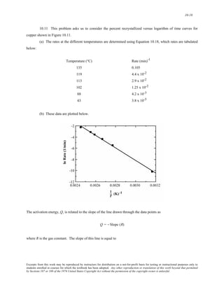

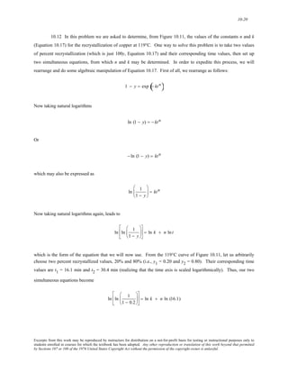


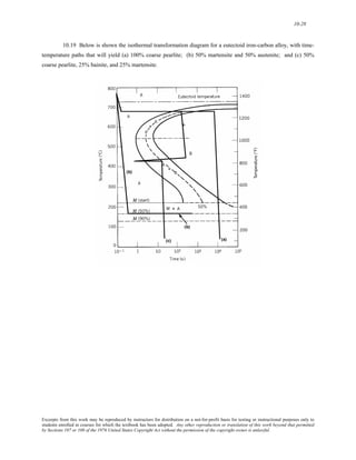


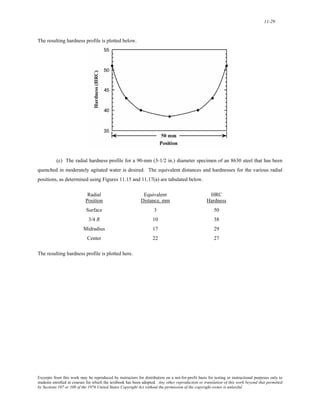
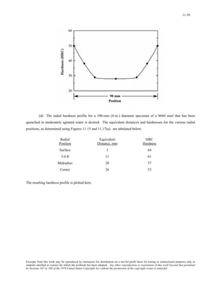
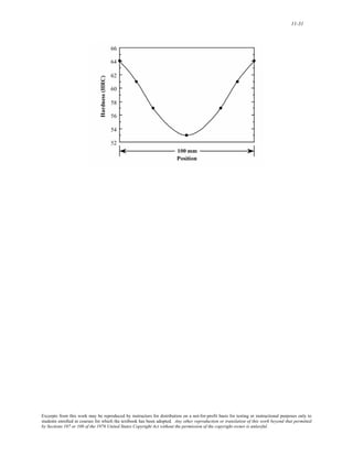
![11-32
11.29 We are asked to compare the effectiveness of quenching in moderately agitated water and oil by
graphing, on a single plot, the hardness profiles for 75-mm (3-in.) diameter cylindrical specimens of an 8640 steel
that had been quenched in both media.
For moderately agitated water, the equivalent distances and hardnesses for the several radial positions
[Figures 11.17(a) and 11.15] are tabulated below.
Radial Equivalent HRC
Position Distance, mm Hardness
Surface 3 56
3/4 R 8 53
Midradius 13 47
Center 17 42.5
While for moderately agitated oil, the equivalent distances and hardnesses for the several radial positions [Figures
11.17(b) and 11.15] are tabulated below.
Radial Equivalent HRC
Position Distance, mm Hardness
Surface 13 47
3/4 R 19 41.5
Midradius 22 38
Center 25 36
These data are plotted here.
Excerpts from this work may be reproduced by instructors for distribution on a not-for-profit basis for testing or instructional purposes only to
students enrolled in courses for which the textbook has been adopted. Any other reproduction or translation of this work beyond that permitted
by Sections 107 or 108 of the 1976 United States Copyright Act without the permission of the copyright owner is unlawful.](https://image.slidesharecdn.com/ecyluo1ys2qvoutji72q-signature-9b381c5777758ee4fe884904ded9f35d0b251da572c8ac51c821cb24bd095f1b-poli-141018125101-conversion-gate02/85/solution-for-Materials-Science-and-Engineering-7th-edition-by-William-D-Callister-Jr-563-320.jpg)


![11-42
Heat Treatment of Steels
11.D6 A 38-mm (1-1/2 in.) diameter steel specimen is to be quenched in moderately agitated oil. We are
to decide which of five different steels will have surface and center hardnesses of at least 50 and 40 HRC,
respectively.
In moderately agitated oil, the equivalent distances from the quenched end for a 38 mm diameter bar for
surface and center positions are 5 mm (3/16 in.) and 12 mm (15/32 in.), respectively [Figure 11.17(b)]. The
hardnesses at these two positions for the alloys cited (as determined using Figure 11.14) are given below.
Surface Center
Alloy Hardness (HRC) Hardness (HRC)
1040 40 24
5140 53 42
4340 57 55
4140 56 53
8640 55 48
Thus, alloys 4340, 4140, 8640, and 5140 will satisfy the criteria for both surface and center hardnesses.
Excerpts from this work may be reproduced by instructors for distribution on a not-for-profit basis for testing or instructional purposes only to
students enrolled in courses for which the textbook has been adopted. Any other reproduction or translation of this work beyond that permitted
by Sections 107 or 108 of the 1976 United States Copyright Act without the permission of the copyright owner is unlawful.](https://image.slidesharecdn.com/ecyluo1ys2qvoutji72q-signature-9b381c5777758ee4fe884904ded9f35d0b251da572c8ac51c821cb24bd095f1b-poli-141018125101-conversion-gate02/85/solution-for-Materials-Science-and-Engineering-7th-edition-by-William-D-Callister-Jr-573-320.jpg)
![11-43
11.D7 (a) This problem calls for us to decide which of 8660, 8640, 8630, and 8620 alloys may be
fabricated into a cylindrical piece 57 mm (2-1/4 in.) in diameter which, when quenched in mildly agitated water,
will produce a minimum hardness of 45 HRC throughout the entire piece.
The center of the steel cylinder will cool the slowest and therefore will be the softest. In moderately
agitated water the equivalent distance from the quenched end for a 57 mm diameter bar for the center position is
about 11 mm (7/16 in.) [Figure 11.17(a)]. The hardnesses at this position for the alloys cited (Figure 11.15) are
given below.
Center
Alloy Hardness (HRC)
8660 61
8640 49
8630 36
8620 25
Therefore, only 8660 and 8640 alloys will have a minimum of 45 HRC at the center, and therefore, throughout the
entire cylinder.
(b) This part of the problem asks us to do the same thing for moderately agitated oil. In moderately
agitated oil the equivalent distance from the quenched end for a 57 mm diameter bar at the center position is about
17.5 mm (11.16 in.) [Figure 11.17(b)]. The hardnesses at this position for the alloys cited (Figure 11.15) are given
below.
Center
Alloy Hardness (HRC)
8660 59
8640 42
8630 30
8620 21
Therefore, only the 8660 alloy will have a minimum of 45 HRC at the center, and therefore, throughout the entire
cylinder.
Excerpts from this work may be reproduced by instructors for distribution on a not-for-profit basis for testing or instructional purposes only to
students enrolled in courses for which the textbook has been adopted. Any other reproduction or translation of this work beyond that permitted
by Sections 107 or 108 of the 1976 United States Copyright Act without the permission of the copyright owner is unlawful.](https://image.slidesharecdn.com/ecyluo1ys2qvoutji72q-signature-9b381c5777758ee4fe884904ded9f35d0b251da572c8ac51c821cb24bd095f1b-poli-141018125101-conversion-gate02/85/solution-for-Materials-Science-and-Engineering-7th-edition-by-William-D-Callister-Jr-574-320.jpg)
![11-44
11.D8 A forty-four millimeter (one and three-quarter inch) diameter cylindrical steel specimen is to be
heat treated such that the microstructure throughout will be at least 50% martensite. We are to decide which of
several alloys will satisfy this criterion if the quenching medium is moderately agitated (a) oil, and (b) water.
(a) Since the cooling rate is lowest at the center, we want a minimum of 50% martensite at the center
position. From Figure 11.17(b), the cooling rate is equal to an equivalent distance from the quenched end of 13 mm
(9/16 in.). According to Figure 11.14, the hardness corresponding to 50% martensite for these alloys is 42 HRC.
Thus, all we need do is to determine which of the alloys have a 42 HRC hardness at an equivalent distance from the
quenched end of 13 mm (9/16 in.). At an equivalent distance of 13 mm, the following hardnesses are determined
from Figure 11.14 for the various alloys.
Alloy Hardness (HRC)
4340 55
4140 52
8640 47
5140 41
1040 23
Thus, only alloys 4340, 4140 and 8640 will qualify.
(b) For moderately agitated water, the cooling rate at the center of a 44 mm (1-3/4 in.) diameter specimen
is 9 mm (11/32 in.) equivalent distance from the quenched end [Figure 11.17(a)]. At this position, the following
hardnesses are determined from Figure 11.14 for the several alloys.
Alloy Hardness (HRC)
4340 57
4140 55
8640 53
5140 48
1040 30
It is still necessary to have a hardness of 42 HRC or greater at the center; thus, alloys 4340, 4140, 8640, and 5140
qualify.
Excerpts from this work may be reproduced by instructors for distribution on a not-for-profit basis for testing or instructional purposes only to
students enrolled in courses for which the textbook has been adopted. Any other reproduction or translation of this work beyond that permitted
by Sections 107 or 108 of the 1976 United States Copyright Act without the permission of the copyright owner is unlawful.](https://image.slidesharecdn.com/ecyluo1ys2qvoutji72q-signature-9b381c5777758ee4fe884904ded9f35d0b251da572c8ac51c821cb24bd095f1b-poli-141018125101-conversion-gate02/85/solution-for-Materials-Science-and-Engineering-7th-edition-by-William-D-Callister-Jr-575-320.jpg)
![11-45
11.D9 A fifty-millimeter (two-inch) diameter cylindrical steel specimen is to be quenched in moderately
agitated water. We are to decide which of eight different steels will have surface and center hardnesses of at least
50 and 40 HRC, respectively.
In moderately agitated water, the equivalent distances from the quenched end for a 50-mm diameter bar for
surface and center positions are 2 mm (1/16 in.) and 10 mm (3/8 in.), respectively [Figure 11.17(a)]. The
hardnesses at these two positions for the alloys cited are given below (as determined from Figures 11.14 and 11.15).
Surface Center
Alloy Hardness (HRC) Hardness (HRC)
1040 50 27
5140 56 45
4340 57 56
4140 57 54
8620 42 27
8630 51 38
8640 57 51
8660 64 64
Thus, alloys 5140, 4340, 4140, 8640, and 8660 will satisfy the criteria for both surface hardness (minimum 50
HRC) and center hardness (minimum 40 HRC).
Excerpts from this work may be reproduced by instructors for distribution on a not-for-profit basis for testing or instructional purposes only to
students enrolled in courses for which the textbook has been adopted. Any other reproduction or translation of this work beyond that permitted
by Sections 107 or 108 of the 1976 United States Copyright Act without the permission of the copyright owner is unlawful.](https://image.slidesharecdn.com/ecyluo1ys2qvoutji72q-signature-9b381c5777758ee4fe884904ded9f35d0b251da572c8ac51c821cb24bd095f1b-poli-141018125101-conversion-gate02/85/solution-for-Materials-Science-and-Engineering-7th-edition-by-William-D-Callister-Jr-576-320.jpg)


![11-51
11.D15 We are asked to specify a practical heat treatment for a 2014 aluminum alloy that will produce a
minimum yield strength of 345 MPa (50,000 psi), and a minimum ductility of 12%EL. From Figure 11.27(a), the
following heat treating temperatures and time ranges are possible to the give the required yield strength.
Temperature (°C) Time Range (h)
260 not possible
204 0.3-15
149 10-700
121 300-?
With regard to temperatures and times to give the desired ductility [Figure 11.27(b)]:
Temperature (°C) Time Range (h)
260 <0.02, >10
204 <0.4, >350
149 <20
121 <1000
From these tabulations, the following may be concluded:
It is not possible to heat treat this alloy at 260°C so as to produce the desired set of properties—attainment
of a yield strength of 345 MPa is not possible at this temperature.
At204°C, the heat treating time would need to be about 0.4 h, which is practical.
At149°C, the time range is between 10 and 20 h, which is a little on the long side.
Finally, at 121°C, the time range is unpractically long (300 to 1000 h).
Excerpts from this work may be reproduced by instructors for distribution on a not-for-profit basis for testing or instructional purposes only to
students enrolled in courses for which the textbook has been adopted. Any other reproduction or translation of this work beyond that permitted
by Sections 107 or 108 of the 1976 United States Copyright Act without the permission of the copyright owner is unlawful.](https://image.slidesharecdn.com/ecyluo1ys2qvoutji72q-signature-9b381c5777758ee4fe884904ded9f35d0b251da572c8ac51c821cb24bd095f1b-poli-141018125101-conversion-gate02/85/solution-for-Materials-Science-and-Engineering-7th-edition-by-William-D-Callister-Jr-582-320.jpg)


![12-3
There will also be an anion located at the corner, point F (not drawn), and the cube diagonal AEF will be related to
the ionic radii as
AEF = 2(rA + rC)
(The line AEF has not been drawn to avoid confusion.) From the triangle ABF
(AB)2 + (FB)2 = (AEF)2
But,
FB = a =
2rA
2
and
AB = 2rA
from above. Thus,
(2rA)2 +
2rA
2
⎛
⎜
⎝
⎞
⎟
⎠
2
= [2(rA + rC)]2
Solving for the rC/rA ratio leads to
rC
rA
=
6 − 2
2
= 0.225
Excerpts from this work may be reproduced by instructors for distribution on a not-for-profit basis for testing or instructional purposes only to
students enrolled in courses for which the textbook has been adopted. Any other reproduction or translation of this work beyond that permitted
by Sections 107 or 108 of the 1976 United States Copyright Act without the permission of the copyright owner is unlawful.](https://image.slidesharecdn.com/ecyluo1ys2qvoutji72q-signature-9b381c5777758ee4fe884904ded9f35d0b251da572c8ac51c821cb24bd095f1b-poli-141018125101-conversion-gate02/85/solution-for-Materials-Science-and-Engineering-7th-edition-by-William-D-Callister-Jr-586-320.jpg)
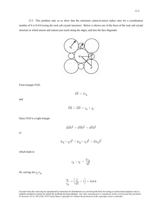


![12-8
12.7 This problem asks that we compute the atomic packing factor for the rock salt crystal structure when
rC/rA = 0.414. From Equation 3.2
APF =
VS
VC
With regard to the sphere volume, VS, there are four cation and four anion spheres per unit cell. Thus,
VS = (4) 4
3
π rA 3
⎛
⎜
⎝
⎞
⎠
⎛ 3
⎝
⎟ + (4) 4
3
π rC
⎜
⎞
⎟
⎠
But, since rC/rA = 0.414
VS = 16
3
π rA 3
1 + (0.414)3 [ ]= (17.94) rA 3
Now, for rC/rA = 0.414 the corner anions in Table 12.2 just touch one another along the cubic unit cell edges such
that
V C = a3 = [2(rA + rC)]3
= 2(rA + 0.414rA) [ ]3 = (22.62) rA 3
Thus
APF =
VS
VC
=
(17.94) rA 3
(22.62) rA 3
= 0.79
Excerpts from this work may be reproduced by instructors for distribution on a not-for-profit basis for testing or instructional purposes only to
students enrolled in courses for which the textbook has been adopted. Any other reproduction or translation of this work beyond that permitted
by Sections 107 or 108 of the 1976 United States Copyright Act without the permission of the copyright owner is unlawful.](https://image.slidesharecdn.com/ecyluo1ys2qvoutji72q-signature-9b381c5777758ee4fe884904ded9f35d0b251da572c8ac51c821cb24bd095f1b-poli-141018125101-conversion-gate02/85/solution-for-Materials-Science-and-Engineering-7th-edition-by-William-D-Callister-Jr-591-320.jpg)

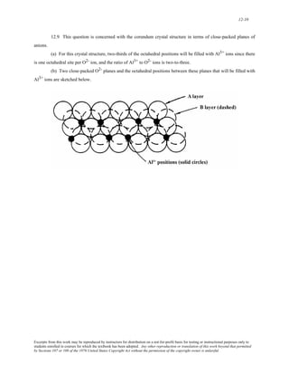

![12-14
In Step 3, we may specify which atoms are to be represented as being bonded to one another, and which
type of bond(s) to use (single solid, single dashed, double, and triple are possibilities), or we may elect to not
represent any bonds at all (in which case we click on the “Go to Step 4” button). If it is decided to show bonds,
probably the best thing to do is to represent unit cell edges as bonds.
The window in Step 4 presents all the data that have been entered; you may review these data for
accuracy. If any changes are required, it is necessary to close out all windows back to the one in which corrections
are to be made, and then reenter data in succeeding windows. When you are fully satisfied with your data, click on
the “Generate” button, and the image that you have defined will be displayed. The image may then be rotated by
using mouse click-and-drag.
Your image should appear as follows:
Here the darker spheres represent oxygen ions, while lead ions are depicted by the lighter balls.
[Note: Unfortunately, with this version of the Molecular Definition Utility, it is not possible to save either the data
or the image that you have generated. You may use screen capture (or screen shot) software to record and store
your image.]
Excerpts from this work may be reproduced by instructors for distribution on a not-for-profit basis for testing or instructional purposes only to
students enrolled in courses for which the textbook has been adopted. Any other reproduction or translation of this work beyond that permitted
by Sections 107 or 108 of the 1976 United States Copyright Act without the permission of the copyright owner is unlawful.](https://image.slidesharecdn.com/ecyluo1ys2qvoutji72q-signature-9b381c5777758ee4fe884904ded9f35d0b251da572c8ac51c821cb24bd095f1b-poli-141018125101-conversion-gate02/85/solution-for-Materials-Science-and-Engineering-7th-edition-by-William-D-Callister-Jr-597-320.jpg)
![12-15
12.13 We are asked to calculate the theoretical density of NiO. This density may be computed using
Equation (12.1) as
ρ =
n'(ANi + AO)
VC NA
Since the crystal structure is rock salt, n' = 4 formula units per unit cell. Using the ionic radii for Ni2+ and O2- from
Table 12.3, the unit cell volume is computed as follows:
VC = a3 = 2r
Ni2+ + 2r
O2-
⎛
⎝
⎜ ⎞
⎟
⎠
3
= [2 (0.069 nm) + 2 (0.140 nm)]3
= 0.0730 nm3
unit cell
= 7.30 x 10⁻²³ cm3
unit cell
Thus,
ρ = (4 formula units/unit cell)(58.69 g/mol + 16.00 g/mol)
(7.30 x 10⁻²³ cm3/unit cell)(6.023 x 10²³ formula units/mol)
= 6.79 g/cm3
Excerpts from this work may be reproduced by instructors for distribution on a not-for-profit basis for testing or instructional purposes only to
students enrolled in courses for which the textbook has been adopted. Any other reproduction or translation of this work beyond that permitted
by Sections 107 or 108 of the 1976 United States Copyright Act without the permission of the copyright owner is unlawful.](https://image.slidesharecdn.com/ecyluo1ys2qvoutji72q-signature-9b381c5777758ee4fe884904ded9f35d0b251da572c8ac51c821cb24bd095f1b-poli-141018125101-conversion-gate02/85/solution-for-Materials-Science-and-Engineering-7th-edition-by-William-D-Callister-Jr-598-320.jpg)


![12-19
12.16 This problem asks that we compute the theoretical density of ZnS given that the Zn—S distance and
bond angle are 0.234 nm and 109.5°, respectively. The first thing we need do is to determine the unit cell volume
from the given Zn—S distance. From the previous problem, the unit cell volume VC is just a3, a being the unit cell
edge length, and
V C = (4y sin θ)3 = [(4)(0.234 nm)(sin 35.25°)]3
= 0.1576 nm3 = 1.576 x 10⁻²² cm3
Now we must utilize Equation 12.1 with n' = 4 formula units, and AZn and AS being 65.39 and 32.06 g/mol,
respectively. Thus
ρ =
n'Ź(AZn + AS)
VC NA
= (4 formula units/unit cell)(65.39 g/mol + 32.06 g/mol)
(1.576 x 10⁻²² cm3/unit cell)(6.023 x 10²³ formula units/mol)
= 4.11 g/cm3
The measured value of the density is 4.10 g/cm3.
Excerpts from this work may be reproduced by instructors for distribution on a not-for-profit basis for testing or instructional purposes only to
students enrolled in courses for which the textbook has been adopted. Any other reproduction or translation of this work beyond that permitted
by Sections 107 or 108 of the 1976 United States Copyright Act without the permission of the copyright owner is unlawful.](https://image.slidesharecdn.com/ecyluo1ys2qvoutji72q-signature-9b381c5777758ee4fe884904ded9f35d0b251da572c8ac51c821cb24bd095f1b-poli-141018125101-conversion-gate02/85/solution-for-Materials-Science-and-Engineering-7th-edition-by-William-D-Callister-Jr-602-320.jpg)
![12-20
12.17 We are asked to determine the number of Si4+ and O2- ions per unit cell for a crystalline form of
silica (SiO2). For this material, a = 0.700 nm and ρ = 2.32 g/cm3. Solving for n ' from Equation 12.1, we get
n' =
ρVCNA
ASi + 2AO
=
ρa3NA
ASi + 2AO
= (2.32g /cm3)(7.00 x 10−8cm)3(6.023 x 10²³ formula units / mol)
(28.09g /mol + 2[16.00]g / mol)
= 7.98 or almost 8
Therefore, there are eight Si4+ and sixteen O2- per unit cell.
Excerpts from this work may be reproduced by instructors for distribution on a not-for-profit basis for testing or instructional purposes only to
students enrolled in courses for which the textbook has been adopted. Any other reproduction or translation of this work beyond that permitted
by Sections 107 or 108 of the 1976 United States Copyright Act without the permission of the copyright owner is unlawful.](https://image.slidesharecdn.com/ecyluo1ys2qvoutji72q-signature-9b381c5777758ee4fe884904ded9f35d0b251da572c8ac51c821cb24bd095f1b-poli-141018125101-conversion-gate02/85/solution-for-Materials-Science-and-Engineering-7th-edition-by-William-D-Callister-Jr-603-320.jpg)
![12-22
12.19 This problem asks that we compute the density of CaF2. A unit cell of the fluorite structure is
shown in Figure 12.5. It may be seen that there are four CaF2 units per unit cell (i.e., n' = 4 formula units/unit cell).
Assume that for each of the eight small cubes in the unit cell
a =
2r
Ca2+ + 2r
F−
3
and, from Table 12.3
a = 2 (0.100 nm) + 2 (0.133 nm)
3
= 0.269 nm = 2.69 x 10⁻⁸ cm
The volume of the unit cell is just
VC = (2a)3 = [(2)(2.69 x 10⁻³ cm)]3
= 1.56 x 10⁻²² cm3
Thus, from Equation 12.1
ρ =
n'Ź( ACa + 2AF)
VC NA
= (4 formula units/unit cell)[40.08 g/mol + (2)(19.00 g/mol)]
(1.56 x 10⁻²² cm3/unit cell)( 6.023 x 10²³ formula units/mol)
= 3.33 g/cm3
The measured density is 3.18 g/cm3.
Excerpts from this work may be reproduced by instructors for distribution on a not-for-profit basis for testing or instructional purposes only to
students enrolled in courses for which the textbook has been adopted. Any other reproduction or translation of this work beyond that permitted
by Sections 107 or 108 of the 1976 United States Copyright Act without the permission of the copyright owner is unlawful.](https://image.slidesharecdn.com/ecyluo1ys2qvoutji72q-signature-9b381c5777758ee4fe884904ded9f35d0b251da572c8ac51c821cb24bd095f1b-poli-141018125101-conversion-gate02/85/solution-for-Materials-Science-and-Engineering-7th-edition-by-William-D-Callister-Jr-605-320.jpg)

(30.0 + 28.5) g/mol
= 4.00 formula units/unit cell
Of the three possible crystal structures, only sodium chloride and zinc blende have four formula units per unit cell,
and therefore, are possibilities.
Excerpts from this work may be reproduced by instructors for distribution on a not-for-profit basis for testing or instructional purposes only to
students enrolled in courses for which the textbook has been adopted. Any other reproduction or translation of this work beyond that permitted
by Sections 107 or 108 of the 1976 United States Copyright Act without the permission of the copyright owner is unlawful.](https://image.slidesharecdn.com/ecyluo1ys2qvoutji72q-signature-9b381c5777758ee4fe884904ded9f35d0b251da572c8ac51c821cb24bd095f1b-poli-141018125101-conversion-gate02/85/solution-for-Materials-Science-and-Engineering-7th-edition-by-William-D-Callister-Jr-606-320.jpg)

(3)(55.85 g/mol) + (4)(16.00 g/mol)
= 8.0 formula units/unit cell
Thus, in each unit cell there are 8 Fe2+, 16 Fe3+, and 32 O2- ions. From Table 12.3, rFe2+ = 0.077 nm, rFe3+ =
0.069 nm, and rO2- = 0.140 nm. Thus, the total sphere volume in Equation 3.2 (which we denote as VS), is just
VS = (8) 4
3
π
⎛
⎜
⎝
⎞
⎠
⎟ (7.7 x 10⁻⁹cm)3 + (16) 4
3
π
⎛
⎜
⎝
⎞
⎠
⎟ (6.9 x 10⁻⁹cm)3
+ (32) 4
3
π
⎛
⎜
⎝
⎞
⎠
⎟ (1.40 x 10⁻⁸ cm)3
= 4.05 x 10⁻²² cm3
Now, the unit cell volume (VC) is just
V C = a3 = (8.39 x 10⁻⁸ cm)3 = 5.90 x 10⁻²² cm3
Finally, the atomic packing factor (APF) from Equation 3.2 is just
APF =
VS
VC
= 4.05 x 10⁻²² cm3
5.90 x 10⁻²² cm3 = 0.686
Excerpts from this work may be reproduced by instructors for distribution on a not-for-profit basis for testing or instructional purposes only to
students enrolled in courses for which the textbook has been adopted. Any other reproduction or translation of this work beyond that permitted
by Sections 107 or 108 of the 1976 United States Copyright Act without the permission of the copyright owner is unlawful.](https://image.slidesharecdn.com/ecyluo1ys2qvoutji72q-signature-9b381c5777758ee4fe884904ded9f35d0b251da572c8ac51c821cb24bd095f1b-poli-141018125101-conversion-gate02/85/solution-for-Materials-Science-and-Engineering-7th-edition-by-William-D-Callister-Jr-607-320.jpg)

![12-27
12.23 We are asked in this problem to compute the atomic packing factor for the diamond cubic crystal
structure, given that the angle between adjacent bonds is 109.5°. The first thing that we must do is to determine the
unit cell volume VC in terms of the atomic radius r. From Problem 12.15 the following relationship was developed
a = 4y sin θ
in which y = 2r and θ = 35.25°. Furthermore, since the unit cell is cubic, VC = a3; therefore
V C = (4y sin θ)3 = [(4)(2r)(sin 35.25°)]3 = 98.43 r3
Now, it is necessary to determine the sphere volume in the unit cell, VS, in terms of r. For this unit cell (Figure
12.15) there are 4 interior atoms, 6 face atoms, and 8 corner atoms. The entirety of the interior atoms, one-half of
each face atom, and one-eighth of each corner atom belong to the unit cell. Therefore, there are 8 equivalent atoms
per unit cell; hence
π r3 ⎛
⎝
VS = (8) 4
3
⎜
⎞
⎠
⎟ = 33.51 r3
Finally, the atomic packing factor is just
APF =
VS
VC
= 33.51 r3
98.43 r3 = 0.340
Excerpts from this work may be reproduced by instructors for distribution on a not-for-profit basis for testing or instructional purposes only to
students enrolled in courses for which the textbook has been adopted. Any other reproduction or translation of this work beyond that permitted
by Sections 107 or 108 of the 1976 United States Copyright Act without the permission of the copyright owner is unlawful.](https://image.slidesharecdn.com/ecyluo1ys2qvoutji72q-signature-9b381c5777758ee4fe884904ded9f35d0b251da572c8ac51c821cb24bd095f1b-poli-141018125101-conversion-gate02/85/solution-for-Materials-Science-and-Engineering-7th-edition-by-William-D-Callister-Jr-610-320.jpg)
![12-28
12.24 We are asked in this problem to compute the atomic packing factor for the CsCl crystal structure.
This requires that we take the ratio of the sphere volume within the unit cell and the total unit cell volume. From
Figure 12.3 there is the equivalence of one Cs and one Cl ion per unit cell; the ionic radii of these two ions are
0.170 nm and 0.181 nm, respectively (Table 12.3). Thus, the sphere volume, VS, is just
VS = 4
3
(π)[(0.170 nm)3 + (0.181 nm)3] = 0.0454 nm3
For CsCl the unit cell edge length, a, in terms of the atomic radii is just
a =
2r
Cs+ + 2r
Cl-
3
= 2(0.170 nm) + 2(0.181 nm)
3
= 0.405 nm
Since VC = a3
VC = (0.405 nm)3 = 0.0664 nm3
And, finally the atomic packing factor is just
APF =
VS
VC
= 0.0454 nm3
0.0664 nm3 = 0.684
Excerpts from this work may be reproduced by instructors for distribution on a not-for-profit basis for testing or instructional purposes only to
students enrolled in courses for which the textbook has been adopted. Any other reproduction or translation of this work beyond that permitted
by Sections 107 or 108 of the 1976 United States Copyright Act without the permission of the copyright owner is unlawful.](https://image.slidesharecdn.com/ecyluo1ys2qvoutji72q-signature-9b381c5777758ee4fe884904ded9f35d0b251da572c8ac51c821cb24bd095f1b-poli-141018125101-conversion-gate02/85/solution-for-Materials-Science-and-Engineering-7th-edition-by-William-D-Callister-Jr-611-320.jpg)
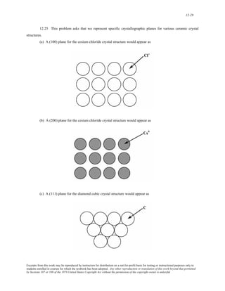


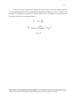


![12-54
Miscellaneous Mechanical Considerations
12.46 (a) This portion of the problem requests that we compute the modulus of elasticity for nonporous
spinel given that E = 240 GPa for a material having 5 vol% porosity. Thus, we solve Equation 12.9 for E0, using P
= 0.05, which gives
E0 = E
1 − 1.9P + 0.9P2
= 240 GPa
1 − (1.9)(0.05) + (0.9)(0.05)2 = 265 GPa (38.6 x 10⁶ psi)
(b) Now we are asked to determine the value of E at P = 15 vol% (i.e., 0.15). Using Equation 12.9 we get
E = E0(1 − 1.9P + 0.9P2)
= (265 GPa)[1 − (1.9)(0.15) + (0.09)(0.15)2]= 195 GPa (28.4 x 10⁶ psi)
Excerpts from this work may be reproduced by instructors for distribution on a not-for-profit basis for testing or instructional purposes only to
students enrolled in courses for which the textbook has been adopted. Any other reproduction or translation of this work beyond that permitted
by Sections 107 or 108 of the 1976 United States Copyright Act without the permission of the copyright owner is unlawful.](https://image.slidesharecdn.com/ecyluo1ys2qvoutji72q-signature-9b381c5777758ee4fe884904ded9f35d0b251da572c8ac51c821cb24bd095f1b-poli-141018125101-conversion-gate02/85/solution-for-Materials-Science-and-Engineering-7th-edition-by-William-D-Callister-Jr-637-320.jpg)

![12-57
12.49 (a) Given the flexural strengths at two different volume fraction porosities, we are asked to
determine the flexural strength for a nonporous material. If the natural logarithm is taken of both sides of Equation
12.10, then
lnσ fs = lnσ0 − nP
Using the data provided in the problem statement, two simultaneous equations may be written as
ln (70 MPa) = ln σ0 − (0.10) n
ln (60 MPa) = ln σ0 − (0.15) n
Solving for n and σ0 leads to n = 3.08 and σ0 = 95.3 MPa. For the nonporous material, P = 0, and, from Equation
12.10, σ0 = σfs. Thus, σfs for P = 0 is 95.3 MPa.
(b) Now, we are asked for σfs at P = 0.20 for this same material. Utilizing Equation 12.10 yields
σ fs = σ0 exp (− nP)
= (95.3 MPa) exp [− (3.08)(0.20)]
= 51.5 MPa
Excerpts from this work may be reproduced by instructors for distribution on a not-for-profit basis for testing or instructional purposes only to
students enrolled in courses for which the textbook has been adopted. Any other reproduction or translation of this work beyond that permitted
by Sections 107 or 108 of the 1976 United States Copyright Act without the permission of the copyright owner is unlawful.](https://image.slidesharecdn.com/ecyluo1ys2qvoutji72q-signature-9b381c5777758ee4fe884904ded9f35d0b251da572c8ac51c821cb24bd095f1b-poli-141018125101-conversion-gate02/85/solution-for-Materials-Science-and-Engineering-7th-edition-by-William-D-Callister-Jr-640-320.jpg)


![13-4
13.4 (a) From Figure 12.25, for a spinel-bonded magnesia material (88.5 wt%MgO-11.5 wt% Al2O3), the
maximum temperature without a liquid phase corresponds to the temperature at the MgO(ss)-[MgO(ss) + Liquid]
boundary at this composition, which is approximately 2220°C (4030°F).
(b) The maximum temperature without the formation of a liquid phase for a magnesia-alumina spinel (25
wt%MgO-75 wt% Al2O3) lies at the phase boundary between MgAl2O4(ss)-(MgAl2O4 + Liquid) phase fields (just
slightly to the right of the congruent melting point at which the two phase boundaries become tangent); this
temperature is approximately 2070°C (3760°F).
Excerpts from this work may be reproduced by instructors for distribution on a not-for-profit basis for testing or instructional purposes only to
students enrolled in courses for which the textbook has been adopted. Any other reproduction or translation of this work beyond that permitted
by Sections 107 or 108 of the 1976 United States Copyright Act without the permission of the copyright owner is unlawful.](https://image.slidesharecdn.com/ecyluo1ys2qvoutji72q-signature-9b381c5777758ee4fe884904ded9f35d0b251da572c8ac51c821cb24bd095f1b-poli-141018125101-conversion-gate02/85/solution-for-Materials-Science-and-Engineering-7th-edition-by-William-D-Callister-Jr-647-320.jpg)
![13-5
13.5 For each section of this problem two SiO2-Al2O3 compositions are given; we are to decide, on the
basis of the SiO2-Al2O3 phase diagram (Figure 12.27), which is the more desirable refractory and then justify the
choice.
(a) The 99.8 wt% SiO2-0.2 wt% Al2O3 will be more desirable because the liquidus temperature will be
greater for this composition; therefore, at any temperature within the cristobalite + liquid region on the phase
diagram, there will be a lower fraction of the liquid phase present than for the 99.0 wt% SiO2-1.0 wt% Al2O3
composition, and, thus, the mechanical integrity will be greater.
(b) The 74 wt% Al2O3-26 wt% SiO2 composition will be more desirable because, for this composition, a
liquid phase does not form until about 1750°C [i.e., the temperature at which a vertical line at 74 wt% Al2O3
crosses the boundary between the mullite and (mullite + liquid) phase regions]; for the 70 wt% Al2O3-30 wt%
SiO2 material, a liquid phase forms at a much lower temperature--1587°C.
(c) The 95 wt% Al2O3-5 wt% SiO2 composition will be more desirable because the liquidus temperature
will be greater for this composition. Therefore, at any temperature within the alumina + liquid region on the phase
diagram, there will be a lower fraction of the liquid phase present than for the 90 wt% Al2O3-10 wt% SiO2
composition, and, thus, the mechanical integrity of the 95 wt% Al2O3-5 wt% SiO2 material will be greater.
Excerpts from this work may be reproduced by instructors for distribution on a not-for-profit basis for testing or instructional purposes only to
students enrolled in courses for which the textbook has been adopted. Any other reproduction or translation of this work beyond that permitted
by Sections 107 or 108 of the 1976 United States Copyright Act without the permission of the copyright owner is unlawful.](https://image.slidesharecdn.com/ecyluo1ys2qvoutji72q-signature-9b381c5777758ee4fe884904ded9f35d0b251da572c8ac51c821cb24bd095f1b-poli-141018125101-conversion-gate02/85/solution-for-Materials-Science-and-Engineering-7th-edition-by-William-D-Callister-Jr-648-320.jpg)


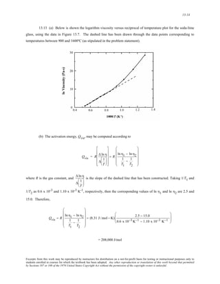


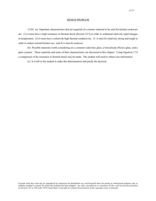

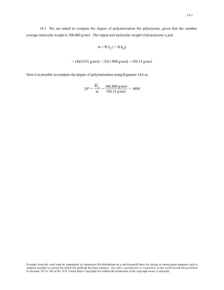


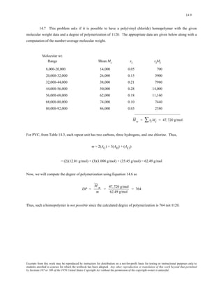
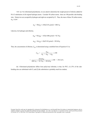


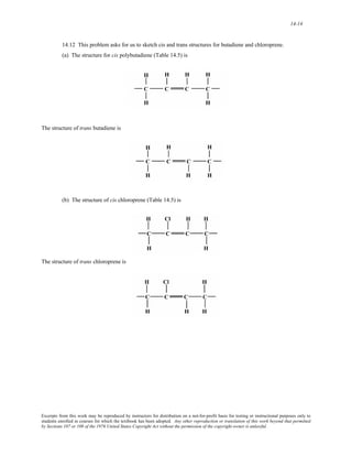


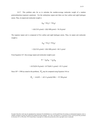
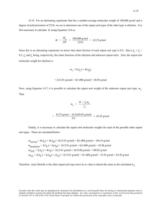

![14-23
14.21 For a random poly(styrene-butadiene) copolymer in which M n = 350,000 g/mol and DP = 5000, we
are asked to compute the fractions of styrene and butadiene repeat units.
From Table 14.5, the styrene repeat unit has eight carbon and eight hydrogen atoms. Thus,
mst = (8)(12.01 g/mol) + (8)(1.008 g/mol) = 104.14 g/mol
Also, from Table 14.5, the butadiene repeat unit has four carbon and six hydrogen atoms, and
mbu = (4)(12.01 g/mol) + (6)(1.008 g/mol) = 54.09 g/mol
From Equation 14.7
m = fstmst + fbumbu
Now, let x = fst, such that
m = 104.14x + (54.09)(1 − x)
since fst + fbu = 1. Also, from Equation 14.6
DP =
M n
m
Or
5000 = 350,000 g /mol
[104.14 x + 54.09(1 − x)] g /mol
Solving for x leads to x = fst = f(styrene) = 0.32. Also,
f(butadiene) = 1 – x = 1 – 0.32 = 0.68
Excerpts from this work may be reproduced by instructors for distribution on a not-for-profit basis for testing or instructional purposes only to
students enrolled in courses for which the textbook has been adopted. Any other reproduction or translation of this work beyond that permitted
by Sections 107 or 108 of the 1976 United States Copyright Act without the permission of the copyright owner is unlawful.](https://image.slidesharecdn.com/ecyluo1ys2qvoutji72q-signature-9b381c5777758ee4fe884904ded9f35d0b251da572c8ac51c821cb24bd095f1b-poli-141018125101-conversion-gate02/85/solution-for-Materials-Science-and-Engineering-7th-edition-by-William-D-Callister-Jr-693-320.jpg)

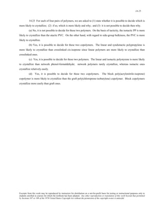


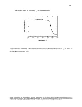


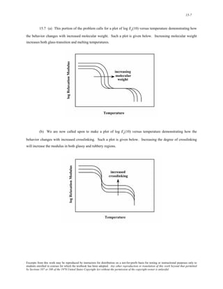


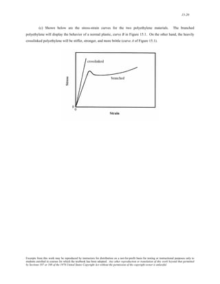


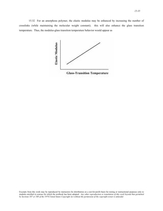


![15-40
15.37 (a) This problem asks that we determine how much ethylene glycol must be added to 20.0 kg of
terephthalic acid to produce a linear chain structure of poly(ethylene terephthalate) according to Equation 15.9.
Since the chemical formulas are provided in this equation we may calculate the molecular weights of each of these
materials as follows:
MW(ethylene glycol) = 2( AC) + 6( AH) + 2( AO)
= 2(12.01 g/mol) + 6(1.008 g/mol) + 2(16.00 g/mol) = 62.07 g/mol
MW(terephthalic acid) = 8(AC) + 6(AH) + 4(AO)
= 8 (12.01 g/mol) + 6(1.008 g/mol) + 4(16.00 g/mol) = 166.13 g/mol
The 20.0 kg mass of terephthalic acid equals 20,000 g or
20,000 g
166.13 g /mol
= 120.39 mol. Since, according to
Equation 15.9, each mole of terephthalic acid used requires one mole of ethylene glycol, which is equivalent to
(120.39 mol)(62.07 g/mol) = 7473 g = 7.473 kg.
(b) Now we are asked for the mass of the resulting polymer. Inasmuch as one mole of water is given off
for every repeat unit produced, this corresponds to 120.39 moles or (120.39 mol)(18.02 g/mol) = 2169 g or 2.169 kg
since the molecular weight of water is 18.02 g/mol. The mass of poly(ethylene terephthalate) is just the sum of the
masses of the two reactant materials [as computed in part (a)] minus the mass of water released, or
mass [poly(ethylene terephthalate)] = 20.0 kg + 7.473 kg − 2.169 kg = 25.304 kg
Excerpts from this work may be reproduced by instructors for distribution on a not-for-profit basis for testing or instructional purposes only to
students enrolled in courses for which the textbook has been adopted. Any other reproduction or translation of this work beyond that permitted
by Sections 107 or 108 of the 1976 United States Copyright Act without the permission of the copyright owner is unlawful.](https://image.slidesharecdn.com/ecyluo1ys2qvoutji72q-signature-9b381c5777758ee4fe884904ded9f35d0b251da572c8ac51c821cb24bd095f1b-poli-141018125101-conversion-gate02/85/solution-for-Materials-Science-and-Engineering-7th-edition-by-William-D-Callister-Jr-743-320.jpg)


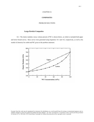
![16-3
16.3 Given the elastic moduli and specific gravities for copper and tungsten we are asked to estimate the
upper limit for specific stiffness when the volume fractions of tungsten and copper are 0.70 and 0.30, respectively.
There are two approaches that may be applied to solve this problem. The first is to estimate both the upper limits of
elastic modulus [Ec(u)] and specific gravity (ρc) for the composite, using expressions of the form of Equation 16.1,
and then take their ratio. Using this approach
Ec(u) = ECuVCu + EWVW
= (110 GPa)(0.30) + (407 GPa)(0.70)
= 318 GPa
And
ρc = ρCuVCu + ρWVW
= (8.9)(0.30) + (19.3)(0.70) = 16.18
Therefore
Specific Stiffness =
Ec (u)
ρc
= 318 GPa
16.18
= 19.65 GPa
With the alternate approach, the specific stiffness is calculated, again employing a modification of
Equation 16.1, but using the specific stiffness-volume fraction product for both metals, as follows:
Specific Stiffness =
ECu
ρCu
VCu +
EW
ρW
VW
= 110 GPa
8.9
(0.30) + 407 GPa
19.3
(0.70) = 18.47 GPa
Excerpts from this work may be reproduced by instructors for distribution on a not-for-profit basis for testing or instructional purposes only to
students enrolled in courses for which the textbook has been adopted. Any other reproduction or translation of this work beyond that permitted
by Sections 107 or 108 of the 1976 United States Copyright Act without the permission of the copyright owner is unlawful.](https://image.slidesharecdn.com/ecyluo1ys2qvoutji72q-signature-9b381c5777758ee4fe884904ded9f35d0b251da572c8ac51c821cb24bd095f1b-poli-141018125101-conversion-gate02/85/solution-for-Materials-Science-and-Engineering-7th-edition-by-William-D-Callister-Jr-756-320.jpg)


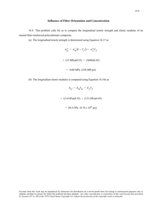


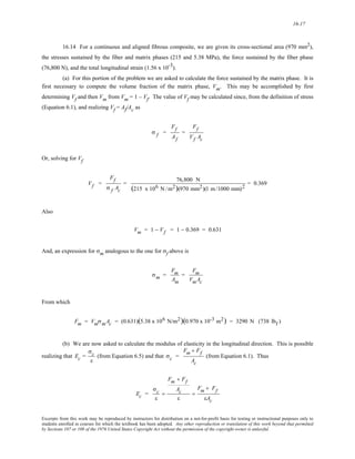


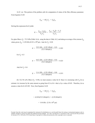
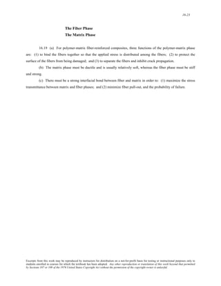


![16-38
Influence of Fiber Orientation and Concentration
16.D2 In order to solve this problem, we want to make longitudinal elastic modulus and tensile strength
computations assuming 40 vol% fibers for all three fiber materials, in order to see which meet the stipulated criteria
[i.e., a minimum elastic modulus of 55 GPa (8 x 10⁶ psi), and a minimum tensile strength of 1200 MPa (175,000
psi)]. Thus, it becomes necessary to use Equations 16.10b and 16.17 with Vm = 0.6 and Vf = 0.4, Em = 3.1 GPa, and
= 69 MPa. σm ∗
For glass, Ef = 72.5 GPa and = 3450 MPa. Therefore, σf ∗
Ecl = Em(1 − Vf ) + Ef Vf
= (3.1 GPa)(1 − 0.4) + (72.5 GPa)(0.4) = 30.9 GPa (4.48 x 10⁶ psi)
Since this is less than the specified minimum (i.e., 55 GPa), glass is not an acceptable candidate.
For carbon (PAN standard-modulus), Ef = 230 GPa and = 4000 MPa (the average of the range of
values in Table B.4), thus, from Equation 16.10b
σf ∗
Ecl = (3.1 GPa)(0.6) + (230 GPa)(0.4) = 93.9 GPa (13.6 x 10⁶ psi)
which is greater than the specified minimum. In addition, from Equation 16.17
∗ = σmÕ(1 − Vf ) + σf ∗
σcl
Vf
= (30 MPa)(0.6) + (4000 MPa)(0.4) = 1620 MPa (234, 600 psi)
which is also greater than the minimum (1200 MPa). Thus, carbon (PAN standard-modulus) is a candidate.
For aramid, Ef = 131 GPa and = 3850 MPa (the average of the range of values in Table B.4), thus
(Equation 16.10b)
σf ∗
Ecl = (3.1 GPa)(0.6) + (131 GPa)(0.4) = 54.3 GPa (7.87 x 10⁶ psi)
Excerpts from this work may be reproduced by instructors for distribution on a not-for-profit basis for testing or instructional purposes only to
students enrolled in courses for which the textbook has been adopted. Any other reproduction or translation of this work beyond that permitted
by Sections 107 or 108 of the 1976 United States Copyright Act without the permission of the copyright owner is unlawful.](https://image.slidesharecdn.com/ecyluo1ys2qvoutji72q-signature-9b381c5777758ee4fe884904ded9f35d0b251da572c8ac51c821cb24bd095f1b-poli-141018125101-conversion-gate02/85/solution-for-Materials-Science-and-Engineering-7th-edition-by-William-D-Callister-Jr-791-320.jpg)


![16-43
= (0.35)(0.015 x 10⁻³ m)
(4)(80 MPa)(5 x 10⁻³ m) = 3.28 x 10⁻⁶ (MPa)-1 [2.23 x 10⁻⁸ (psi)−1]
Furthermore,
b = −Vf = − 0.35
And
∗ − σm
c = σcd
' (1 − Vf )
= 1200 MPa − (6.55 MPa)(1 − 0.35) = 1195.74 MPa (174,383 psi)
Now solving the above quadratic equation for yields σf ∗
σf ∗
=
− b ± b2 − 4ac
2a
=
− (−0.35) ± (−0.35)2 − (4)[3.28 x 10⁻⁶ (MPa)−1](1195.74 MPa)
(2)[3.28 x 10⁻⁶ (MPa)−1]
6.56 x 10⁻⁶ MPa 0.3500 ± 0.3270
= 0.3500 ± 0.3268
4.46 x 10⁻⁸ psi
⎡
⎢
⎣
⎢
⎤
⎥
⎦
⎥
This yields the two possible roots as
σf ∗
(+) = 0.3500 + 0.3268
6.56 x 10⁻⁶ MPa = 103,200 MPa (15.2 x 10⁶ psi)
σf ∗
(−) = 0.3500 − 0.3268
6.56 x 10⁻⁶ MPa = 3537 MPa (515,700 psi)
σf ∗
σf ∗
(−)
Upon consultation of the magnitudes of for various fibers and whiskers in Table 16.4, only is
reasonable. Now, using this value, let us calculate the value of lc using Equation 16.3 in order to ascertain if use of
Equation 16.18 in the previous treatment was appropriate. Thus
Excerpts from this work may be reproduced by instructors for distribution on a not-for-profit basis for testing or instructional purposes only to
students enrolled in courses for which the textbook has been adopted. Any other reproduction or translation of this work beyond that permitted
by Sections 107 or 108 of the 1976 United States Copyright Act without the permission of the copyright owner is unlawful.](https://image.slidesharecdn.com/ecyluo1ys2qvoutji72q-signature-9b381c5777758ee4fe884904ded9f35d0b251da572c8ac51c821cb24bd095f1b-poli-141018125101-conversion-gate02/85/solution-for-Materials-Science-and-Engineering-7th-edition-by-William-D-Callister-Jr-796-320.jpg)


![17-4
17.4 (a) We are asked to compute the voltage of a nonstandard Pb-Sn electrochemical cell. Since tin is
lower in the standard emf series (Table 17.1), we will begin by assuming that tin is oxidized and lead is reduced, as
Sn + Pb2+ → Sn2+ + Pb
and Equation 17.20 takes the form
D − VSn
ΔV = (VPb
D ) − 0.0592
2
log [Sn2+ ]
[Pb2+ ]
= [−0.126 V − (−0.136 V)] − 0.0592
2
log 0.25
5 x 10⁻²
⎡
⎢
⎣
⎢
⎤
⎥
⎦
⎥
= – 0.011 V
since, from Table 17.1, the standard potentials for Pb and Sn are –0.126 and –0.136, respectively.
(b) Since the ΔV is negative, the spontaneous cell direction is just the reverse of that above, or
Sn2+ + Pb → Sn + Pb2+
Excerpts from this work may be reproduced by instructors for distribution on a not-for-profit basis for testing or instructional purposes only to
students enrolled in courses for which the textbook has been adopted. Any other reproduction or translation of this work beyond that permitted
by Sections 107 or 108 of the 1976 United States Copyright Act without the permission of the copyright owner is unlawful.](https://image.slidesharecdn.com/ecyluo1ys2qvoutji72q-signature-9b381c5777758ee4fe884904ded9f35d0b251da572c8ac51c821cb24bd095f1b-poli-141018125101-conversion-gate02/85/solution-for-Materials-Science-and-Engineering-7th-edition-by-William-D-Callister-Jr-803-320.jpg)
![17-5
17.5 This problem calls for us to determine whether or not a voltage is generated in a Fe/Fe2+
2 concentration cell, 2
and, if so, its magnitude. Let us label the Fe cell having a 0.5 M Fe2+ solution as cell 1, and the
other as cell 2. Furthermore, assume that oxidation occurs within cell 2, wherein [Fe+ ] = 2 x 10⁻² M. Hence,
2+ → Fe2
Fe2 + Fe1
2+ + Fe1
and, employing Equation 17.20 leads to
ΔV = − 0.0592
2
log
[ 2 2
Fe+]
Fe1
[ 2+]
= − 0.0592
2
log 2 x 10⁻² M
0.5M
⎡
⎢
⎣
⎢
⎤
⎥
⎦
⎥
= + 0.0414 V
Therefore, a voltage of 0.0414 V is generated when oxidation occurs in the cell 2, the one having a Fe2+
concentration of 2 x 10⁻² M.
Excerpts from this work may be reproduced by instructors for distribution on a not-for-profit basis for testing or instructional purposes only to
students enrolled in courses for which the textbook has been adopted. Any other reproduction or translation of this work beyond that permitted
by Sections 107 or 108 of the 1976 United States Copyright Act without the permission of the copyright owner is unlawful.](https://image.slidesharecdn.com/ecyluo1ys2qvoutji72q-signature-9b381c5777758ee4fe884904ded9f35d0b251da572c8ac51c821cb24bd095f1b-poli-141018125101-conversion-gate02/85/solution-for-Materials-Science-and-Engineering-7th-edition-by-William-D-Callister-Jr-804-320.jpg)
![17-6
17.6 We are asked to calculate the concentration of Cu2+ ions in a copper-cadmium electrochemical cell.
The electrochemical reaction that occurs within this cell is just
Cd + Cu2+ → Cd2+ + Cu
while ΔV = 0.775 V and [Cd2+] = 6.5 x 10⁻² M. Thus, Equation 17.20 is written in the form
ΔV = (VCu
D ) − 0.0592
D − VCd
2
log [Cd2+ ]
[Cu2+ ]
This equation may be rewritten as
−
ΔV − (VCu
D )
D − VCd
0.0296
= log [Cd2+ ]
[Cu2+ ]
Solving this expression for [Cu2+] gives
[Cu2+] = [Cd2+] exp + (2.303)
ΔV − (VCu
D )
D −VPb
0.0296
⎡
⎢
⎣
⎢
⎤
⎥
⎦
⎥
D = +0.340 V and V = – 0.403 V. Therefore, Cd
The standard potentials from Table 17.1 are VCu
D
[Cu2+] = (6.5 x 10⁻² M) exp+ (2.303)
0.775 V − {0.340 V − (−0.403 V)}
0.0296
⎡
⎢
⎣
⎤
⎥
⎦
= 0.784 M
Excerpts from this work may be reproduced by instructors for distribution on a not-for-profit basis for testing or instructional purposes only to
students enrolled in courses for which the textbook has been adopted. Any other reproduction or translation of this work beyond that permitted
by Sections 107 or 108 of the 1976 United States Copyright Act without the permission of the copyright owner is unlawful.](https://image.slidesharecdn.com/ecyluo1ys2qvoutji72q-signature-9b381c5777758ee4fe884904ded9f35d0b251da572c8ac51c821cb24bd095f1b-poli-141018125101-conversion-gate02/85/solution-for-Materials-Science-and-Engineering-7th-edition-by-William-D-Callister-Jr-805-320.jpg)
![17-7
17.7 This problem asks for us to calculate the temperature for a zinc-lead electrochemical cell when the
potential between the Zn and Pb electrodes is +0.568 V. On the basis of their relative positions in the standard emf
series (Table 17.1), assume that Zn is oxidized and Pb is reduced. Thus, the electrochemical reaction that occurs
within this cell is just
Pb2+ + Zn → Pb + Zn2+
Thus, Equation 17.20 is written in the form
ΔV = (VPb
D ) − RT
D − VZn
nF
ln [Zn2+ ]
[Pb2+ ]
Solving this expression for T gives
T = − nF
R
ΔV − (VPb
D )
D −VZn
ln [Zn2+ ]
[Pb2+ ]
⎡
⎢
⎢
⎢
⎢
⎢
⎣
⎤
⎥
⎥
⎥
⎥
⎥
⎦
D VPb
D
The standard potentials from Table 17.1 are V Zn = – 0.763 V and = – 0.126 V. Therefore,
T = − (2)(96,500 C/mol)
8.31 J /mol - K
0.568 V−{−0.126 V− (−0.763 V)}
⎛
⎝
10−2 ln ⎜⎜
M
10−4 M
⎞
⎟⎟
⎠
⎡
⎢
⎢
⎢
⎢
⎢
⎣
⎤
⎥
⎥
⎥
⎥
⎥
⎦
= 348 K = 75°C
Excerpts from this work may be reproduced by instructors for distribution on a not-for-profit basis for testing or instructional purposes only to
students enrolled in courses for which the textbook has been adopted. Any other reproduction or translation of this work beyond that permitted
by Sections 107 or 108 of the 1976 United States Copyright Act without the permission of the copyright owner is unlawful.](https://image.slidesharecdn.com/ecyluo1ys2qvoutji72q-signature-9b381c5777758ee4fe884904ded9f35d0b251da572c8ac51c821cb24bd095f1b-poli-141018125101-conversion-gate02/85/solution-for-Materials-Science-and-Engineering-7th-edition-by-William-D-Callister-Jr-806-320.jpg)

![17-10
Corrosion Rates
17.10 This problem is just an exercise in unit conversions. The parameter K in Equation 17.23 must
convert the units of W, ρ, A, and t, into the unit scheme for the CPR.
For CPR in mpy (mil/yr)
K = W(mg)(1 g /1000 mg)
⎛
⎝
ρ g
⎜
cm3
⎞
⎟
⎠
2.54 cm
in.
⎛
⎜
⎝
⎞
⎟
⎠
3
⎡ A(in.2)
⎢⎣
⎤
⎥⎦
1 in.
1000 mil
⎛
⎜
⎝
⎞
⎠
⎟[ t(h)] 1 day
24 h
⎛
⎜
⎝
⎞
⎟
⎠
1 yr
365 days
⎛
⎜
⎝
⎞
⎟
⎠
= 534.6
For CPR in mm/yr
K = W(mg)(1 g /1000 mg)
⎛
⎝
ρ g
⎜
cm3
⎞
⎟
⎠
1 cm
10 mm
⎛
⎜
⎝
⎞
⎟
⎠
3
⎡ A(cm2)
⎢⎣
⎤
⎥⎦
10 mm
cm
⎛
⎜
⎝
⎞
⎟
⎠
2
[t(h)] 1 day
24 h
⎛
⎜
⎝
⎞
⎟
⎠
1 yr
365 days
⎛
⎜
⎝
⎞
⎟
⎠
= 87.6
Excerpts from this work may be reproduced by instructors for distribution on a not-for-profit basis for testing or instructional purposes only to
students enrolled in courses for which the textbook has been adopted. Any other reproduction or translation of this work beyond that permitted
by Sections 107 or 108 of the 1976 United States Copyright Act without the permission of the copyright owner is unlawful.](https://image.slidesharecdn.com/ecyluo1ys2qvoutji72q-signature-9b381c5777758ee4fe884904ded9f35d0b251da572c8ac51c821cb24bd095f1b-poli-141018125101-conversion-gate02/85/solution-for-Materials-Science-and-Engineering-7th-edition-by-William-D-Callister-Jr-809-320.jpg)


![17-18
17.17 (a) This portion of the problem asks that we compute the rate of oxidation for Ni given that both the
oxidation and reduction reactions are controlled by activation polarization, and also given the polarization data for
both nickel oxidation and hydrogen reduction. The first thing necessary is to establish relationships of the form of
Equation 17.25 for the potentials of both oxidation and reduction reactions. Next we will set these expressions
equal to one another, and then solve for the value of i which is really the corrosion current density, ic. Finally, the
corrosion rate may be calculated using Equation 17.24. The two potential expressions are as follows:
For hydrogen reduction
VH = V
(H+/H2 )
+ βH log i
i0H
⎛
⎜
⎜
⎝
⎞
⎟
⎟
⎠
And for Ni oxidation
VNi= V
(Ni/Ni2+)
+ βNi log i
i0Ni
⎛
⎜
⎜
⎝
⎞
⎟
⎟
⎠
Setting VH = VNi and solving for log i (log ic) leads to
log ic = 1
βNi − βH
⎛
⎜⎜
⎝
⎞
⎠
⎟⎟ V
(H+ /H2 )
− V
(Ni /Ni2+ )
− βH log i0H
+ βNi log i0Ni
⎡
⎢
⎣
⎤
⎥
⎦
And, incorporating values for the various parameters provided in the problem statement leads to
log ic = 1
0.12 − (−0.10)
⎡
⎢
⎣
⎤
⎦
⎥ 0 − (−0.25) − (−0.10){log(6 x10−
[ 7 )} + (0.12){log(10−8)}]
= –6.055
Or
ic = 10-6.055 = 8.81 x 10⁻⁷ A/cm2
And from Equation 17.24
Excerpts from this work may be reproduced by instructors for distribution on a not-for-profit basis for testing or instructional purposes only to
students enrolled in courses for which the textbook has been adopted. Any other reproduction or translation of this work beyond that permitted
by Sections 107 or 108 of the 1976 United States Copyright Act without the permission of the copyright owner is unlawful.](https://image.slidesharecdn.com/ecyluo1ys2qvoutji72q-signature-9b381c5777758ee4fe884904ded9f35d0b251da572c8ac51c821cb24bd095f1b-poli-141018125101-conversion-gate02/85/solution-for-Materials-Science-and-Engineering-7th-edition-by-William-D-Callister-Jr-817-320.jpg)

![17-20
17.18 (a) This portion of the problem asks that we compute the rate of oxidation for a divalent metal M
given that both the oxidation and reduction reactions are controlled by activation polarization, and also given the
polarization data for both M oxidation and hydrogen reduction. The first thing necessary is to establish
relationships of the form of Equation 17.25 for the potentials of both oxidation and reduction reactions. Next we
will set these expressions equal to one another, and then solve for the value of i which is really the corrosion current
density, ic. Finally, the corrosion rate may be calculated using Equation 17.24. The two potential expressions are
as follows:
For hydrogen reduction
VH = V
(H+/H2 )
+ βH log i
i0H
⎛
⎜
⎜
⎝
⎞
⎟
⎟
⎠
And for M oxidation
VM = V
(M/M2+ )
+ βM log i
i0M
⎛
⎜
⎜
⎝
⎞
⎟
⎟
⎠
Setting VH = VM and solving for log i (log ic) leads to
log ic = 1
βM − βH
⎛
⎜⎜
⎝
⎞
⎠
⎟⎟ V
(H+ /H2 )
− V
(M /M2+ )
− βH log i0H
+ βM log i0M
⎡
⎢
⎣
⎤
⎥
⎦
And, incorporating values for the various parameters provided in the problem statement leads to
log ic = 1
0.10 − (−0.15)
⎡
⎢
⎣
⎤
⎦
⎥ [0 − (−0.90) − (−0.15){log(10−10)} + (0.10){log(10−12)}]
= – 7.20
Or
ic = 10-7.20 = 6.31 x 10⁻⁸ A/cm2
And from Equation 17.24
Excerpts from this work may be reproduced by instructors for distribution on a not-for-profit basis for testing or instructional purposes only to
students enrolled in courses for which the textbook has been adopted. Any other reproduction or translation of this work beyond that permitted
by Sections 107 or 108 of the 1976 United States Copyright Act without the permission of the copyright owner is unlawful.](https://image.slidesharecdn.com/ecyluo1ys2qvoutji72q-signature-9b381c5777758ee4fe884904ded9f35d0b251da572c8ac51c821cb24bd095f1b-poli-141018125101-conversion-gate02/85/solution-for-Materials-Science-and-Engineering-7th-edition-by-William-D-Callister-Jr-819-320.jpg)


![17-29
17.25 For a concentration cell, corrosion occurs at that region having the lower concentration. In order to
H L 2
2
explain this phenomenon let us consider an electrochemical cell consisting of two divalent metal M electrodes each
of which is immersed in a solution containing a different concentration of its M2+ ion; let us designate the low and
high concentrations of M2+ as [M+ ] and [M+ ], respectively. Now assuming that reduction and oxidation
reactions occur in the high- and low-concentration solutions, respectively, let us determine the cell potential in terms
of the two [M2+]'s; if this potential is positive then we have chosen the solutions in which the reduction and
oxidation reactions appropriately.
Thus, the two half-reactions in the form of Equations 17.16 are
2+ + 2e- → M V M D
MH
2++ 2e-
M → ML
−VM D
Whereas the overall cell reaction is
2+ + M → M + ML
MH
2+
From Equation 17.19, this yields a cell potential of
ΔV = VM D
− VM D
− RT
nF
ln
[ML 2
+ ]
[MH 2+ ]
⎛
⎜
⎜
⎝
⎞
⎟
⎟
⎠
= − RT
nF
ln
[ML 2
+ ]
[MH 2
+ ]
⎛
⎜
⎜
⎝
⎞
⎟
⎟
⎠
+ ] [M2+ ] ratio is negative, which yields a positive
Inasmuch as [H L 2
2
M+ ] < [Mthen the natural logarithm of the value for ΔV. This means that the electrochemical reaction is spontaneous as written, or that oxidation occurs at the
electrode having the lower M2+ concentration.
Excerpts from this work may be reproduced by instructors for distribution on a not-for-profit basis for testing or instructional purposes only to
students enrolled in courses for which the textbook has been adopted. Any other reproduction or translation of this work beyond that permitted
by Sections 107 or 108 of the 1976 United States Copyright Act without the permission of the copyright owner is unlawful.](https://image.slidesharecdn.com/ecyluo1ys2qvoutji72q-signature-9b381c5777758ee4fe884904ded9f35d0b251da572c8ac51c821cb24bd095f1b-poli-141018125101-conversion-gate02/85/solution-for-Materials-Science-and-Engineering-7th-edition-by-William-D-Callister-Jr-828-320.jpg)


![17-37
K5 + K6 = 10W /K4
For some solvers, using the above expression, the following instructions can be used:
K5 *t1 + K6 = 10^(W1/K4)
K5 *t2 + K6 = 10^(W2/K4)
K5 *t3 + K6 = 10^(W3/K4)
t1 = 100; W1 = 6.16
t2 = 250; W2 = 8.59
t3 = 1000; W3 = 12.72
The resulting solutions—i.e., values for the K parameters—are
K4 = 7.305
K5 = 0.0535
K6 = 1.622
Now solving Equation 17.36 for W at a time of 5000 min
W = K4 log (K5t + K6)
= 7.305 log [(0.0535)(5000 min) + 1.622]
= 17.75 mg/cm2
Excerpts from this work may be reproduced by instructors for distribution on a not-for-profit basis for testing or instructional purposes only to
students enrolled in courses for which the textbook has been adopted. Any other reproduction or translation of this work beyond that permitted
by Sections 107 or 108 of the 1976 United States Copyright Act without the permission of the copyright owner is unlawful.](https://image.slidesharecdn.com/ecyluo1ys2qvoutji72q-signature-9b381c5777758ee4fe884904ded9f35d0b251da572c8ac51c821cb24bd095f1b-poli-141018125101-conversion-gate02/85/solution-for-Materials-Science-and-Engineering-7th-edition-by-William-D-Callister-Jr-836-320.jpg)


 7.0 x 10⁻³ m
2
⎛
⎜⎜
⎝
⎞
⎟⎟
⎠
2 = 121.4 Ω
Excerpts from this work may be reproduced by instructors for distribution on a not-for-profit basis for testing or instructional purposes only to
students enrolled in courses for which the textbook has been adopted. Any other reproduction or translation of this work beyond that permitted
by Sections 107 or 108 of the 1976 United States Copyright Act without the permission of the copyright owner is unlawful.](https://image.slidesharecdn.com/ecyluo1ys2qvoutji72q-signature-9b381c5777758ee4fe884904ded9f35d0b251da572c8ac51c821cb24bd095f1b-poli-141018125101-conversion-gate02/85/solution-for-Materials-Science-and-Engineering-7th-edition-by-William-D-Callister-Jr-843-320.jpg)
![18-2
18.2 For this problem, given that an aluminum wire 10 m long must experience a voltage drop of less than
1.0 V when a current of 5 A passes through it, we are to compute the minimum diameter of the wire. Combining
Equations 18.3 and 18.4 and solving for the cross-sectional area A leads to
A = Il
Vσ
From Table 18.1, for aluminum σ = 3.8 x 10⁷ (Ω-m)-1. Furthermore, inasmuch as
A = π d
2
⎛
⎜
⎝
⎞
⎟
⎠
2
for a cylindrical
wire, then
⎛
⎝
π d
⎜
2
⎞
⎟
⎠
2
= Il
Vσ
or
d = 4 Il
πVσ
When values for the several parameters given in the problem statement are incorporated into this expression, we get
d = (4)(5 A)(10 m)
(π)(1.0 V)[3.8 x 10⁷ (Ω− m)−1]
= 1.3 x 10⁻³ m = 1.3 mm
Excerpts from this work may be reproduced by instructors for distribution on a not-for-profit basis for testing or instructional purposes only to
students enrolled in courses for which the textbook has been adopted. Any other reproduction or translation of this work beyond that permitted
by Sections 107 or 108 of the 1976 United States Copyright Act without the permission of the copyright owner is unlawful.](https://image.slidesharecdn.com/ecyluo1ys2qvoutji72q-signature-9b381c5777758ee4fe884904ded9f35d0b251da572c8ac51c821cb24bd095f1b-poli-141018125101-conversion-gate02/85/solution-for-Materials-Science-and-Engineering-7th-edition-by-William-D-Callister-Jr-844-320.jpg)
 3 x 10⁻³ m
2
⎛
⎜⎜
⎝
⎞
⎟⎟
⎠
2
= 848 m
Excerpts from this work may be reproduced by instructors for distribution on a not-for-profit basis for testing or instructional purposes only to
students enrolled in courses for which the textbook has been adopted. Any other reproduction or translation of this work beyond that permitted
by Sections 107 or 108 of the 1976 United States Copyright Act without the permission of the copyright owner is unlawful.](https://image.slidesharecdn.com/ecyluo1ys2qvoutji72q-signature-9b381c5777758ee4fe884904ded9f35d0b251da572c8ac51c821cb24bd095f1b-poli-141018125101-conversion-gate02/85/solution-for-Materials-Science-and-Engineering-7th-edition-by-William-D-Callister-Jr-845-320.jpg)

 5 x 10⁻³ m
2
⎛
⎜⎜
⎝
⎞
⎟⎟
⎠
2
= 6.7 x 10⁻³ Ω
(b) If V = 0.04 V then, from Equation 18.1
I = V
R
= 0.04 V
6.7 x 10⁻³ Ω
= 6.0 A
(c) The current density is just
J = I
A
= I
π d
2
⎛
⎜
⎝
⎞
⎟
⎠
2 = 6.0 A
3 m
2
⎛
⎝
π 5 x 10−
⎜⎜
⎞
⎟⎟
⎠
2 = 3.06 x 10⁵ A/m2
(d) The electric field is just
E = V
l
= 0.04 V
5 m
= 8.0 x 10⁻³ V/m
Excerpts from this work may be reproduced by instructors for distribution on a not-for-profit basis for testing or instructional purposes only to
students enrolled in courses for which the textbook has been adopted. Any other reproduction or translation of this work beyond that permitted
by Sections 107 or 108 of the 1976 United States Copyright Act without the permission of the copyright owner is unlawful.](https://image.slidesharecdn.com/ecyluo1ys2qvoutji72q-signature-9b381c5777758ee4fe884904ded9f35d0b251da572c8ac51c821cb24bd095f1b-poli-141018125101-conversion-gate02/85/solution-for-Materials-Science-and-Engineering-7th-edition-by-William-D-Callister-Jr-847-320.jpg)


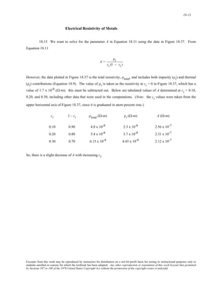

−150°C − (−50°C)
6.5 x 10⁻¹¹ (Ω-m)/°C
and
ρ0 = ρt1 − T1
ρt1 − ρt2
T1 −T2
⎡
⎢
⎣
⎢
⎤
⎥
⎦
⎥
Excerpts from this work may be reproduced by instructors for distribution on a not-for-profit basis for testing or instructional purposes only to
students enrolled in courses for which the textbook has been adopted. Any other reproduction or translation of this work beyond that permitted
by Sections 107 or 108 of the 1976 United States Copyright Act without the permission of the copyright owner is unlawful.](https://image.slidesharecdn.com/ecyluo1ys2qvoutji72q-signature-9b381c5777758ee4fe884904ded9f35d0b251da572c8ac51c821cb24bd095f1b-poli-141018125101-conversion-gate02/85/solution-for-Materials-Science-and-Engineering-7th-edition-by-William-D-Callister-Jr-856-320.jpg)

−150°C − (−50°C)
= 1.58 x 10⁻⁸ (Ω-m)
(b) For this part of the problem, we want to calculate A from Equation 18.11
ρi = Aci (1 − ci )
In Figure 18.8, curves are plotted for three ci values (0.0112, 0.0216, and 0.0332). Let us find A for each of these
ci's by taking a ρtotal from each curve at some temperature (say 0°C) and then subtracting out ρi for pure copper at
this same temperature (which is 1.7 x 10⁻⁸ Ω-m). Below is tabulated values of A determined from these three ci
values, and other data that were used in the computations.
ci 1 – ci ρtotal (Ω-m) ρi (Ω-m) A (Ω-m)
0.0112 0.989 3.0 x 10⁻⁸ 1.3 x 10⁻⁸ 1.17 x 10⁻⁶
0.0216 0.978 4.2 x 10⁻⁸ 2.5 x 10⁻⁸ 1.18 x 10⁻⁶
0.0332 0.967 5.5 x 10⁻⁸ 3.8 x 10⁻⁸ 1.18 x 10⁻⁶
The average of these three A values is 1.18 x 10⁻⁶ (Ω-m).
(c) We use the results of parts (a) and (b) to estimate the electrical resistivity of copper containing 2.50
at% Ni (ci = 0.025) at120°C. The total resistivity is just
ρtotal = ρt + ρi
Or incorporating the expressions for ρt and ρi from Equations 18.10 and 18.11, and the values of ρ0, a, and A
determined above, leads to
ρtotal = (ρ0 + aT) + Aci (1 − ci )
= {1.58 x 10 -8 (Ω - m) + [6.5 x 10 -11 (Ω- m) /°C](120°C)}
+ {[1.18 x 10 -6 (Ω- m)](0.0250) (1 − 0.0250)}
= 5.24 x 10⁻⁸ (Ω-m)
Excerpts from this work may be reproduced by instructors for distribution on a not-for-profit basis for testing or instructional purposes only to
students enrolled in courses for which the textbook has been adopted. Any other reproduction or translation of this work beyond that permitted
by Sections 107 or 108 of the 1976 United States Copyright Act without the permission of the copyright owner is unlawful.](https://image.slidesharecdn.com/ecyluo1ys2qvoutji72q-signature-9b381c5777758ee4fe884904ded9f35d0b251da572c8ac51c821cb24bd095f1b-poli-141018125101-conversion-gate02/85/solution-for-Materials-Science-and-Engineering-7th-edition-by-William-D-Callister-Jr-857-320.jpg)

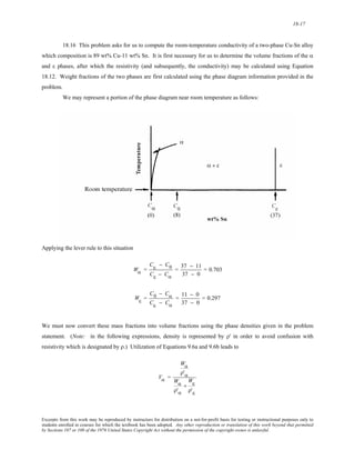


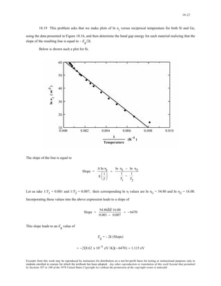


![18-33
18.29 (a) In this problem, for a Si specimen, we are given values for p (2.0 x 10²² m-3) and σ [500 (Ω-
m)-1], while values for μh and μe (0.05 and 0.14 m2/V-s, respectively) are found in Table 18.3. In order to solve
for n we must use Equation 18.13, which, after rearrangement, leads to
n =
σ − p| e | μh
| e | μe
= 500 (Ω − m)−1 − (2.0 x 10²² m−3)(1.602 x 10⁻¹⁹ C)(0.05 m2 /V- s)
(1.602 x 10⁻¹⁹ C)(0.14 m2 /V- s)
= 2.97 x 10²⁰ m-3
(b) This material is p-type extrinsic since p (2.0 x 10²² m-3) is greater than n (2.97 x 10²⁰ m-3).
Excerpts from this work may be reproduced by instructors for distribution on a not-for-profit basis for testing or instructional purposes only to
students enrolled in courses for which the textbook has been adopted. Any other reproduction or translation of this work beyond that permitted
by Sections 107 or 108 of the 1976 United States Copyright Act without the permission of the copyright owner is unlawful.](https://image.slidesharecdn.com/ecyluo1ys2qvoutji72q-signature-9b381c5777758ee4fe884904ded9f35d0b251da572c8ac51c821cb24bd095f1b-poli-141018125101-conversion-gate02/85/solution-for-Materials-Science-and-Engineering-7th-edition-by-William-D-Callister-Jr-875-320.jpg)


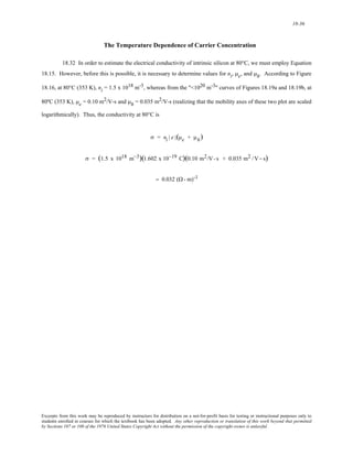
![18-37
18.33 This problem asks for us to assume that electron and hole mobilities for intrinsic Ge are
temperature-dependent, and proportional to T -3/2 for temperature in K. It first becomes necessary to solve for C in
Equation 18.36 using the room-temperature (298 K) conductivity [2.2 (Ω-m)-1] (Table 18.3). This is accomplished
by taking natural logarithms of both sides of Equation 18.36 as
ln σ = ln C − 3
2
lnT −
Eg
2 kT
and after rearranging and substitution of values for Eg (0.67 eV, Table 18.3), and the room-temperature
conductivity, we get
ln C = ln σ + 3
2
lnT +
Eg
2 kT
= ln (2.2) + 3
2
ln (298) + 0.67 eV
(2)(8.62 x 10⁻⁵ eV/K)(298 K)
= 22.38
Now, again using Equation 18.36, we are able to compute the conductivity at 448 K (175°C)
ln σ = ln C − 3
2
ln T −
Eg
2 kT
= 22.38 − 3
2
ln (448 K) − 0.67 eV
(2)(8.62 x 10⁻⁵ eV/K)(448 K)
= 4.548
which leads to
σ = e4.548 = 94.4 (Ω-m)-1.
Excerpts from this work may be reproduced by instructors for distribution on a not-for-profit basis for testing or instructional purposes only to
students enrolled in courses for which the textbook has been adopted. Any other reproduction or translation of this work beyond that permitted
by Sections 107 or 108 of the 1976 United States Copyright Act without the permission of the copyright owner is unlawful.](https://image.slidesharecdn.com/ecyluo1ys2qvoutji72q-signature-9b381c5777758ee4fe884904ded9f35d0b251da572c8ac51c821cb24bd095f1b-poli-141018125101-conversion-gate02/85/solution-for-Materials-Science-and-Engineering-7th-edition-by-William-D-Callister-Jr-879-320.jpg)
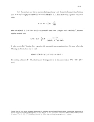
![18-39
18.35 This problem asks that we estimate the temperature at which GaAs has an electrical conductivity of
1.6 x 10⁻³ (Ω-m)-1 assuming that the conductivity has a temperature dependence as shown in Equation 18.36. From
the room temperature (298 K) conductivity [10-6 (Ω-m)-1] and band gap energy (1.42 eV) of Table 18.3 we
determine the value of C (Equation 18.36) by taking natural logarithms of both sides of the equation, and after
rearrangement as follows:
ln C = ln σ + 3
2
ln T +
Eg
2 kT
= ln [10−6 (Ω− m)−1] + 3
2
ln (298 K) + 1.42 eV
(2)(8.62 x 10⁻⁵ eV/K)(298 K)
= 22.37
Now we substitute this value into Equation 18.36 in order to determine the value of T for which σ = 1.6 x 10⁻³ (Ω-
m)-1, thus
ln σ = ln C − 3
2
ln T −
Eg
2 kT
ln [1.6 x 10⁻³ (Ω- m)-1]= 22.37 − 3
2
lnT − 1.42 eV
(2)(8.62 × 10⁻⁵ eV/K) (T)
This equation may be solved for T using an equation solver. For some solvers, the following set of instructions may
be used:
ln(1.6*10^–3) = 22.37 – 1.5*ln(T) – 1.42/(2*8.62*10^–5*T)
The resulting solution is T = 417; this value is the temperature in K which corresponds to T(ºC) = 417 K – 273 =
144°C.
Excerpts from this work may be reproduced by instructors for distribution on a not-for-profit basis for testing or instructional purposes only to
students enrolled in courses for which the textbook has been adopted. Any other reproduction or translation of this work beyond that permitted
by Sections 107 or 108 of the 1976 United States Copyright Act without the permission of the copyright owner is unlawful.](https://image.slidesharecdn.com/ecyluo1ys2qvoutji72q-signature-9b381c5777758ee4fe884904ded9f35d0b251da572c8ac51c821cb24bd095f1b-poli-141018125101-conversion-gate02/85/solution-for-Materials-Science-and-Engineering-7th-edition-by-William-D-Callister-Jr-881-320.jpg)


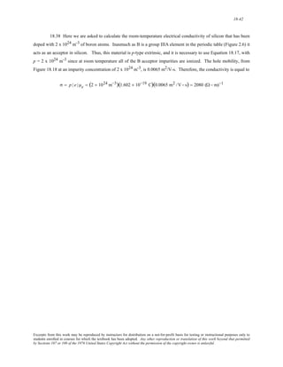


![18-45
The Hall Effect
18.41 (a) This portion of the problem calls for us to determine the electron mobility for some hypothetical
metal using the Hall effect. This metal has an electrical resistivity of 3.3 x 10⁻⁸ (Ω-m), while the specimen
thickness is 15 mm, Ix = 25 A and Bz = 0.95 tesla; under these circumstances a Hall voltage of –2.4 x 10⁻⁷ V is
measured. It is first necessary to convert resistivity to conductivity (Equation 18.4). Thus
σ = 1
ρ
= 1
3.3 x10⁻⁸ (Ω − m)
= 3.0 x 10⁷ (Ω- m)-1
The electron mobility may be determined using Equation 18.20b; and upon incorporation of Equation 18.18, we
have
μe = RH σ
=
VH d σ
I xBz
=
⎛ − 2.4 x 10⁻⁷ V
⎝
⎟( 15 x 10−3 m)[3.0 x 10⁷ (Ω− m)−1]
(25 A)(0.95 tesla)
⎜ ⎞
⎠
= 0.0045 m2/V - s
(b) Now we are to calculate the number of free electrons per cubic meter. From Equation 18.8 we have
n =
σ
| e | μe
= 3.0 x 10⁷ (Ω- m)−1
(1.602 x 10⁻¹⁹ C)(0.0045 m2 /V- s)
= 4.17 x 1028 m-3
Excerpts from this work may be reproduced by instructors for distribution on a not-for-profit basis for testing or instructional purposes only to
students enrolled in courses for which the textbook has been adopted. Any other reproduction or translation of this work beyond that permitted
by Sections 107 or 108 of the 1976 United States Copyright Act without the permission of the copyright owner is unlawful.](https://image.slidesharecdn.com/ecyluo1ys2qvoutji72q-signature-9b381c5777758ee4fe884904ded9f35d0b251da572c8ac51c821cb24bd095f1b-poli-141018125101-conversion-gate02/85/solution-for-Materials-Science-and-Engineering-7th-edition-by-William-D-Callister-Jr-887-320.jpg)

(40 A)(0.0050 m2 /V- s)
⎛ −3.5 x 10⁻⁷ V
⎝
⎜ ⎞
⎠
= 0.74 tesla
Excerpts from this work may be reproduced by instructors for distribution on a not-for-profit basis for testing or instructional purposes only to
students enrolled in courses for which the textbook has been adopted. Any other reproduction or translation of this work beyond that permitted
by Sections 107 or 108 of the 1976 United States Copyright Act without the permission of the copyright owner is unlawful.](https://image.slidesharecdn.com/ecyluo1ys2qvoutji72q-signature-9b381c5777758ee4fe884904ded9f35d0b251da572c8ac51c821cb24bd095f1b-poli-141018125101-conversion-gate02/85/solution-for-Materials-Science-and-Engineering-7th-edition-by-William-D-Callister-Jr-888-320.jpg)


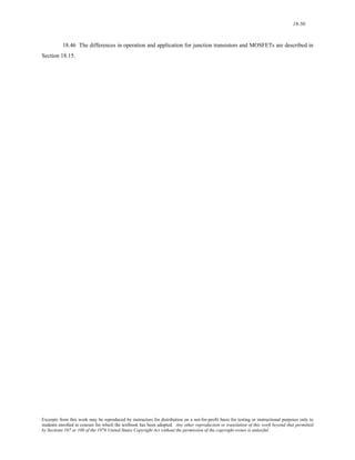


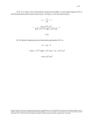


![18-62
18.57 (a) This portion of the problem asks that we compute the magnitude of the dipole moment
associated with each unit cell of BaTiO3, which is illustrated in Figure 18.35. The dipole moment p is defined by
Equation 18.28 as p = qd in which q is the magnitude of each dipole charge, and d is the distance of separation
between the charges. Each Ti4+ ion has four units of charge associated with it, and thus q = (4)(1.602 x 10⁻¹⁹ C) =
6.41 x 10⁻¹⁹ C. Furthermore, d is the distance the Ti4+ ion has been displaced from the center of the unit cell,
which is just 0.006 nm + 0.006 nm = 0.012 nm [Figure 18.35(b)]. Hence
p = qd = (6.41 x 10⁻¹⁹ C)(0.012 x 10 -9 m)
= 7.69 x 10⁻³⁰ C-m
(b) Now it becomes necessary to compute the maximum polarization that is possible for this material. The
maximum polarization will exist when the dipole moments of all unit cells are aligned in the same direction.
Furthermore, it is computed by dividing the above value of p by the volume of each unit cell, which is equal to the
product of three unit cell edge lengths, as shown in Figure 18.35. Thus
P = p
VC
= 7.69 x 10⁻³⁰ C− m
(0.403 x 10⁻⁹ m)(0.398 x 10⁻⁹ m)(0.398 x 10⁻⁹ m)
= 0.121 C/m2
Excerpts from this work may be reproduced by instructors for distribution on a not-for-profit basis for testing or instructional purposes only to
students enrolled in courses for which the textbook has been adopted. Any other reproduction or translation of this work beyond that permitted
by Sections 107 or 108 of the 1976 United States Copyright Act without the permission of the copyright owner is unlawful.](https://image.slidesharecdn.com/ecyluo1ys2qvoutji72q-signature-9b381c5777758ee4fe884904ded9f35d0b251da572c8ac51c821cb24bd095f1b-poli-141018125101-conversion-gate02/85/solution-for-Materials-Science-and-Engineering-7th-edition-by-William-D-Callister-Jr-904-320.jpg)


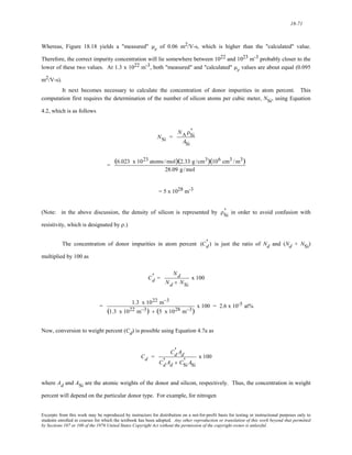
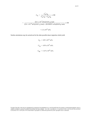
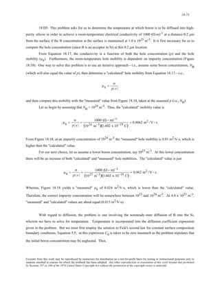
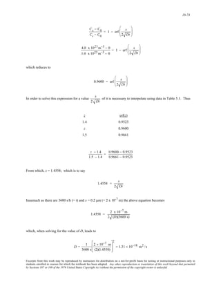
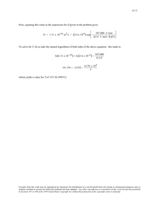
![18-76
Conduction in Ionic Materials
18.D6 This problem asks, for the nonstoichiometric Fe(1 - x)O, given the electrical conductivity [1200 (Ω-
m)-1] and hole mobility (1.0 x 10⁻⁵ m2/V-s) that we determine the value of x. It is first necessary to compute the
number of holes per unit volume (p) using Equation 18.17. Thus
p =
σ
| e | μh
= 1200 (Ω − m)-1
(1.602 × 10⁻¹⁹ C)(1.0 × 10⁻⁵ m2 /V- s) = 7.49 × 1026 holes/m3
Inasmuch as it is assumed that the acceptor states are saturated, the number of vacancies is also 7.49 x 1026 m-3.
Next, it is possible to compute the number of vacancies per unit cell by taking the product of the number of
vacancies per cubic meter times the volume of a unit cell. This volume is just the unit cell edge length (0.437 nm)
cubed:
# vacancies
unit cell
= (7.49 × 1026 m−3)(0.437 x 10⁻⁹m)3 = 0.0625
A unit cell for the sodium chloride structure contains the equivalence of four cations and four anions. Thus, if we
take as a basis for this problem 10 unit cells, there will be 0.625 vacancies, 40 O2- ions, and 39.375 iron ions (since
0.625 of the iron sites is vacant). (It should also be noted that since two Fe3+ ions are created for each vacancy, that
of the 39.375 iron ions, 38.125 of them are Fe2+ and 1.25 of them are Fe3+). In order to find the value of (1 – x) in
the chemical formula, we just take the ratio of the number of total Fe ions (39.375) and the number of total Fe ion
sites (40). Thus
(1 − x) = 39.375
40
= 0.984
Or the formula for this nonstoichiometric material is Fe0.984O.
Excerpts from this work may be reproduced by instructors for distribution on a not-for-profit basis for testing or instructional purposes only to
students enrolled in courses for which the textbook has been adopted. Any other reproduction or translation of this work beyond that permitted
by Sections 107 or 108 of the 1976 United States Copyright Act without the permission of the copyright owner is unlawful.](https://image.slidesharecdn.com/ecyluo1ys2qvoutji72q-signature-9b381c5777758ee4fe884904ded9f35d0b251da572c8ac51c821cb24bd095f1b-poli-141018125101-conversion-gate02/85/solution-for-Materials-Science-and-Engineering-7th-edition-by-William-D-Callister-Jr-918-320.jpg)


![19-3
19.3 (a) This problem asks that we determine the room-temperature heat capacities at constant pressure,
Cp, for copper, iron, gold, and nickel. All we need do is multiply the cp values in Table 19.1 by the atomic weights
(values are found inside the front cover), taking into account the conversion from grams to kilograms (for the
atomic weights). Thus, for Cu
Cp = (386 J/kg - K)(1 kg/1000 g)(63.55 g/mol) = 24.5 J/mol - K
For Fe
Cp = (448 J/kg - K)(1 kg/1000 g)(55.85 g/mol) = 25.0 J/mol - K
For Au
Cp = (128 J/kg - K)(1 kg/1000 g)(196.97 g/mol) = 25.2 J/mol - K
For Ni
Cp = (443 J/kg - K)(1 kg/1000 g)(58.69 g/mol) = 26.0 J/mol - K
(b) These values of Cp are very close to one another because room temperature is considerably above the
Debye temperature for these metals; therefore, the values of Cp should be about equal to 3R [(3)(8.31 J/mol-K) =
24.9 J/mol-K], which is indeed the case for all four of these metals.
Excerpts from this work may be reproduced by instructors for distribution on a not-for-profit basis for testing or instructional purposes only to
students enrolled in courses for which the textbook has been adopted. Any other reproduction or translation of this work beyond that permitted
by Sections 107 or 108 of the 1976 United States Copyright Act without the permission of the copyright owner is unlawful.](https://image.slidesharecdn.com/ecyluo1ys2qvoutji72q-signature-9b381c5777758ee4fe884904ded9f35d0b251da572c8ac51c821cb24bd095f1b-poli-141018125101-conversion-gate02/85/solution-for-Materials-Science-and-Engineering-7th-edition-by-William-D-Callister-Jr-924-320.jpg)


![19-8
19.8 In order to determine the change in length of the copper wire, we must employ a rearranged form of
Equation 19.3b and using the value of αl taken from Table 19.1 [17.0 x 10⁻⁶ (°C)-1] as
Δl = l0αlΔT = l0αl (Tf − T0)
= (15 m)[17.0 x 10⁻⁶ (°C)-1](−9°C − 40°C)
= −1.25 x 10⁻² m = −12.5 mm (−0.49 in.)
Excerpts from this work may be reproduced by instructors for distribution on a not-for-profit basis for testing or instructional purposes only to
students enrolled in courses for which the textbook has been adopted. Any other reproduction or translation of this work beyond that permitted
by Sections 107 or 108 of the 1976 United States Copyright Act without the permission of the copyright owner is unlawful.](https://image.slidesharecdn.com/ecyluo1ys2qvoutji72q-signature-9b381c5777758ee4fe884904ded9f35d0b251da572c8ac51c821cb24bd095f1b-poli-141018125101-conversion-gate02/85/solution-for-Materials-Science-and-Engineering-7th-edition-by-William-D-Callister-Jr-929-320.jpg)

}
= 1.02471 cm3
Thus, the density is just the 7.870 g divided by this new volume—i.e.,
ρ = 7.870 g
1.02471 cm3 = 7.680 g/cm3
Excerpts from this work may be reproduced by instructors for distribution on a not-for-profit basis for testing or instructional purposes only to
students enrolled in courses for which the textbook has been adopted. Any other reproduction or translation of this work beyond that permitted
by Sections 107 or 108 of the 1976 United States Copyright Act without the permission of the copyright owner is unlawful.](https://image.slidesharecdn.com/ecyluo1ys2qvoutji72q-signature-9b381c5777758ee4fe884904ded9f35d0b251da572c8ac51c821cb24bd095f1b-poli-141018125101-conversion-gate02/85/solution-for-Materials-Science-and-Engineering-7th-edition-by-William-D-Callister-Jr-932-320.jpg)
}
= 1.03323 cm3
Thus, the density is just the 19.320 g divided by this new volume—i.e.,
ρ = 19.320 g
1.03323 cm3 = 18.699 g/cm3
(b) Now we are asked to compute the density at 800°C taking into consideration the creation of vacancies
which will further lower the density. To begin, this determination requires that we calculate the number of
vacancies using Equation 4.1. But it first becomes necessary to compute the number of Au atoms per cubic
centimeter (NAu) at 800°C using Equation 4.2. Thus,
NAu =
NA ρAu
AAu
= (6.023 x 10²³atoms /mol)(18.699 g /cm3)
196.97 g /mol
Excerpts from this work may be reproduced by instructors for distribution on a not-for-profit basis for testing or instructional purposes only to
students enrolled in courses for which the textbook has been adopted. Any other reproduction or translation of this work beyond that permitted
by Sections 107 or 108 of the 1976 United States Copyright Act without the permission of the copyright owner is unlawful.](https://image.slidesharecdn.com/ecyluo1ys2qvoutji72q-signature-9b381c5777758ee4fe884904ded9f35d0b251da572c8ac51c821cb24bd095f1b-poli-141018125101-conversion-gate02/85/solution-for-Materials-Science-and-Engineering-7th-edition-by-William-D-Callister-Jr-933-320.jpg)


![19-15
19.13 This problem asks that we calculate the values of cv for aluminum and iron at room temperature
using Equation 19.10, the data in Table 19.1, given that αv = 3αl, and also values of the compressibility. From
Equation 19.10
cv = cp −
2 v0T
β
α v
And, from Table 19.1 and the problem statement
cp(Al) = 900 J/kg-K
cp(Fe) = 448 J/kg-K
αv(Al) = (3)[23.6 x 10⁻⁶ (°C)-1] = 7.08 x 10⁻⁵ (°C)-1
αv(Fe) = (3)[(11.8 x 10⁻⁶ (°C)-1] = 3.54 x 10⁻⁵ (°C)-1
β(Al) = 1.77 x 10⁻¹¹ (Pa)-1
β(Fe) = 2.65 x 10⁻¹² (Pa)-1
The specific volume is just the reciprocal of the density; thus, in units of m3/kg
v0(Al) = 1
ρ
= 1
2.71 g/cm3
⎛
⎜⎜
⎝
⎞
⎟⎟
⎠
1000 g
kg
⎛
⎜
⎝
⎞
⎟
⎠
1 m
100 cm
⎛
⎜
⎝
⎞
⎟
⎠
3
= 3.69 x 10⁻⁴ m3 /kg
v0(Fe) = 1
7.87 g/cm3
⎛
⎜⎜
⎝
⎞
⎟⎟
⎠
1000 g
kg
⎛
⎜
⎝
⎞
⎟
⎠
1 m
100 cm
⎛
⎜
⎝
⎞
⎟
⎠
3
= 1.27 x 10⁻⁴ m3 /kg
Therefore, for aluminum
cv(Al) = cp(Al) −
2(Al) v0(Al)T
α v
β(Al)
= 900 J/kg - K −
⎡ 7.08 x 10⁻⁵ (°C)−1
⎢⎣
⎤
⎥⎦
2
(3.69 x10⁻⁴ m3 /kg) (293 K)
1.77 x 10⁻¹¹ (N /m2)−1
= 869 J/kg-K
And, also for iron
Excerpts from this work may be reproduced by instructors for distribution on a not-for-profit basis for testing or instructional purposes only to
students enrolled in courses for which the textbook has been adopted. Any other reproduction or translation of this work beyond that permitted
by Sections 107 or 108 of the 1976 United States Copyright Act without the permission of the copyright owner is unlawful.](https://image.slidesharecdn.com/ecyluo1ys2qvoutji72q-signature-9b381c5777758ee4fe884904ded9f35d0b251da572c8ac51c821cb24bd095f1b-poli-141018125101-conversion-gate02/85/solution-for-Materials-Science-and-Engineering-7th-edition-by-William-D-Callister-Jr-936-320.jpg)

![19-17
19.14 This problem asks for us to determine the temperature to which a cylindrical rod of tungsten 15.025
mm in diameter must be heated in order for it of just fit into a 15.000 mm diameter circular hole in a plate of 1025
steel (which, of course, is also heated), assuming that the initial temperature is 25°C. This requires the use of
Equation 19.3a, which is applied to the diameters of both the rod and hole. That is
d f − d0
d0
= αl (Tf − T0)
Solving this expression for df yields
d f = d0 1 + αl (T f −T0 ⎡ )
⎢⎣
⎤
⎥⎦
Now all we need do is to establish expressions for df(steel) and df (W), set them equal to one another, and solve for
Tf. According to Table 19.1, αl(steel) = 12.0 x 10⁻⁶ (°C)-1 and αl (W) = 4.5 x 10⁻⁶ (°C)-1. Thus
d f (steel) = d f (W)
(15.000 mm)[1 + {12.0 x 10⁻⁶ (°C)−1}(Tf − 25°C)]
= (15.025 mm)[1 + {4.5 x 10⁻⁶ (°C)−1}(Tf − 25°C)]
Now solving for Tf gives Tf = 222.4°C
Excerpts from this work may be reproduced by instructors for distribution on a not-for-profit basis for testing or instructional purposes only to
students enrolled in courses for which the textbook has been adopted. Any other reproduction or translation of this work beyond that permitted
by Sections 107 or 108 of the 1976 United States Copyright Act without the permission of the copyright owner is unlawful.](https://image.slidesharecdn.com/ecyluo1ys2qvoutji72q-signature-9b381c5777758ee4fe884904ded9f35d0b251da572c8ac51c821cb24bd095f1b-poli-141018125101-conversion-gate02/85/solution-for-Materials-Science-and-Engineering-7th-edition-by-William-D-Callister-Jr-938-320.jpg)


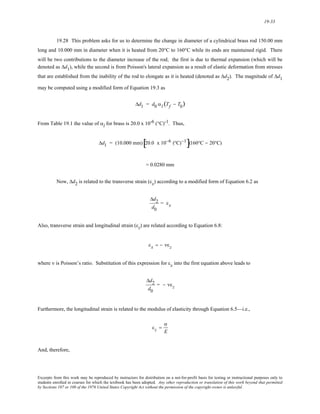


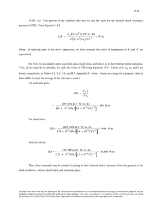
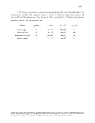


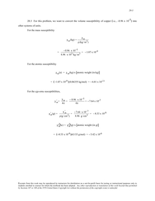


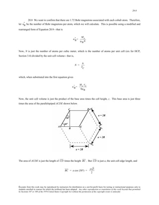
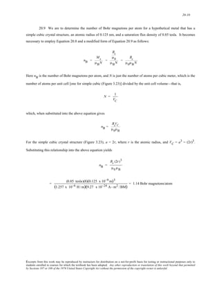
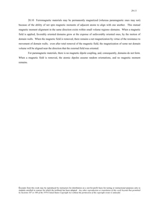
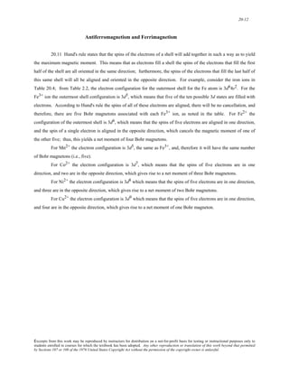
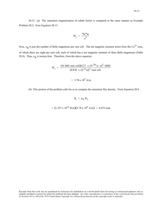


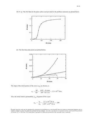


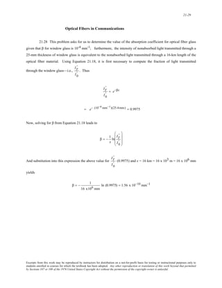

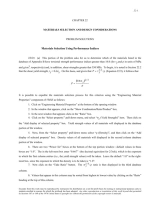
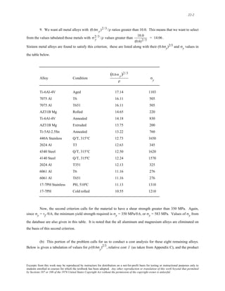

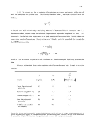


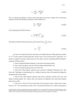


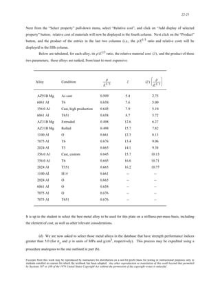


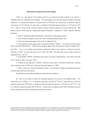
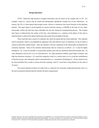

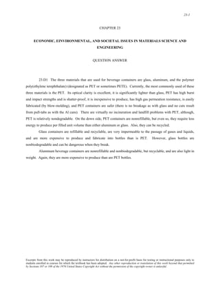

The document discusses several concepts relating to atomic structure and interatomic bonding: 1) It defines atomic mass and atomic weight, and provides an example calculation for the average atomic weight of silicon. 2) It discusses the relationship between atomic mass units (amu) and grams, and derives a conversion factor between the two units. 3) It describes two important concepts from the Bohr model of the atom and two refinements from the wave-mechanical model.


