Download as PDF, PPTX


![Mass Measure
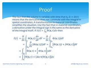
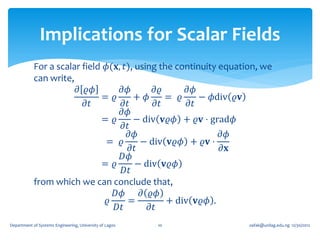
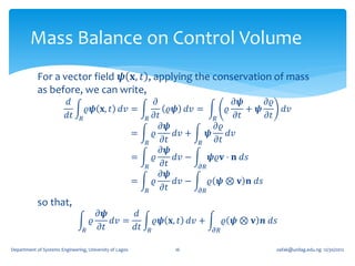
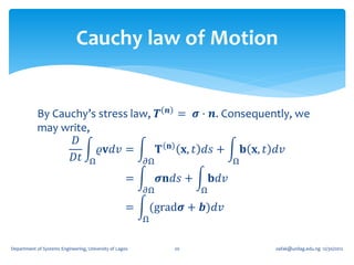
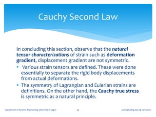
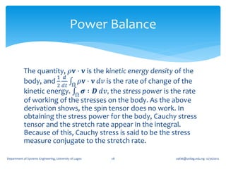
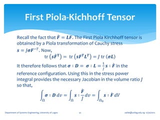
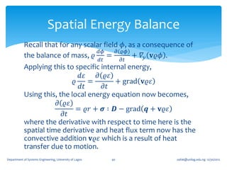
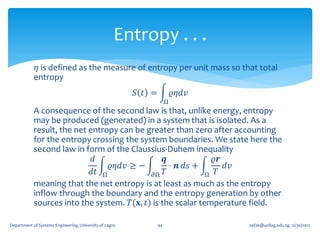
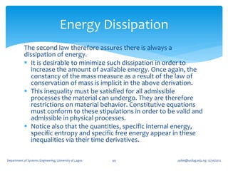
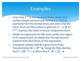
Furthermore, in spatial coordinates, using Leibniz
theorem,
𝐷 𝐷 𝜚𝜙
𝜚𝜙 𝑑𝑣 = + div 𝐯 𝜚𝜙 𝑑𝑣
𝐷𝑡 Ω Ω 𝐷𝑡
𝐷𝜙 𝐷𝜚
= 𝜚 + 𝜙 + 𝜚 div 𝐯) 𝑑𝑣
Ω 𝐷𝑡 𝐷𝑡
𝐷𝜙
= 𝜚 𝑑𝑣
Ω 𝐷𝑡
a relationship we can also arrive at by treating the
“mass measure” 𝜚𝑑𝑣 as a constant under spatial
volume integration [Gurtin et al. pg 130].
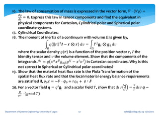
Department of Systems Engineering, University of Lagos 11 oafak@unilag.edu.ng 12/30/2012](https://image.slidesharecdn.com/6-balancelawsjan2013-130103004012-phpapp01/85/6-balance-laws-jan-2013-11-320.jpg)
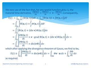
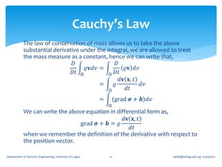
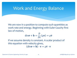
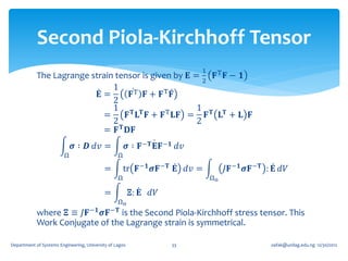
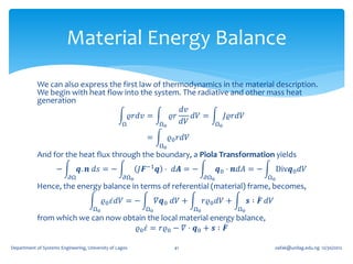
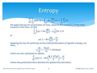
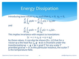
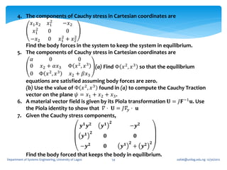
![Vector & Tensor Fields
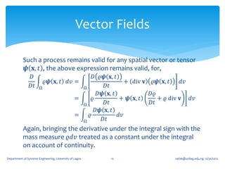
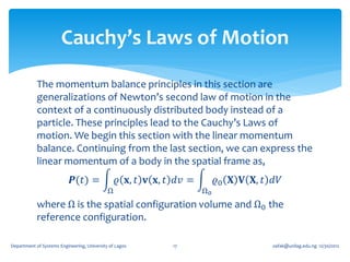
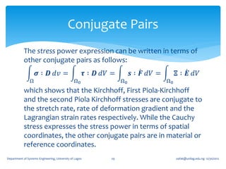
For a vector field 𝝍 𝐱, 𝑡 , we can also write,
𝜕 𝜚𝝍 𝐱, 𝑡 𝜕𝝍 𝜕𝜚 𝜕𝝍
= 𝜚 + 𝝍 = 𝜚 − 𝝍 div 𝐯𝜚
𝜕𝑡 𝜕𝑡 𝜕𝑡 𝜕𝑡
𝜕𝝍 𝜕𝝍
= 𝜚 − div 𝜚𝐯 ⊗ 𝝍 + 𝜚𝐯 ⋅ [See Ex 3.1 28 ]
𝜕𝑡 𝜕𝐱
𝑑𝝍
= 𝜚 − div 𝜚𝐯 ⊗ 𝝍
𝑑𝑡
from which we can conclude that,
𝑑𝝍 𝜕 𝜚𝝍
𝜚 = + div 𝜚𝐯 ⊗ 𝝍
𝑑𝑡 𝜕𝑡
Department of Systems Engineering, University of Lagos 13 oafak@unilag.edu.ng 12/30/2012](https://image.slidesharecdn.com/6-balancelawsjan2013-130103004012-phpapp01/85/6-balance-laws-jan-2013-13-320.jpg)
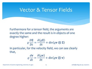
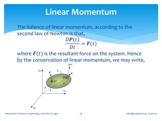
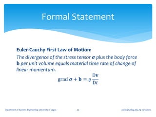
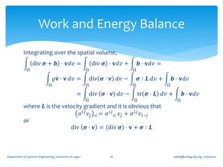
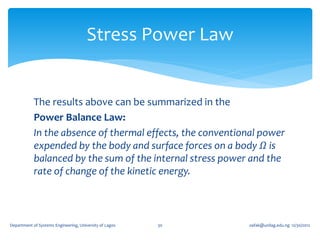
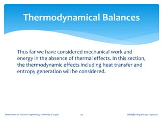
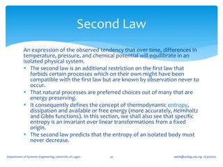
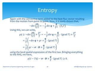
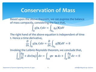
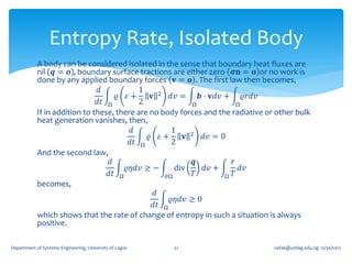
![Free Energy
The Gibbs free energy, originally called available energy, was developed
in the 1870s by the American mathematician Josiah Willard Gibbs. In
1873, Gibbs described this “available energy” as “the greatest amount
of mechanical work which can be obtained from a given quantity of a
certain substance in a given initial state, without increasing its total
volume or allowing heat to pass to or from external bodies, except such
as at the close of the processes are left in their initial condition.” [11] The
initial state of the body, according to Gibbs, is supposed to be such
that "the body can be made to pass from it to states of dissipated energy
by reversible processes." The specific free energy (Gibbs Function) is
defined as 𝜓 = 𝜀 − 𝑇𝜂. Consequently, then we can write,
𝒒
𝜚 𝜓 + 𝑇 𝜂 − 𝝈 ∶ 𝑫 + ⋅ 𝛻 𝑦 𝑇 = −𝑇Γ ≥ 0
𝑇
Department of Systems Engineering, University of Lagos 47 oafak@unilag.edu.ng 12/30/2012](https://image.slidesharecdn.com/6-balancelawsjan2013-130103004012-phpapp01/85/6-balance-laws-jan-2013-47-320.jpg)

The document discusses balance laws in physics, specifically conservation of mass, momentum, and energy. It provides details on: 1) The principle of mass conservation states that the mass of an isolated system remains constant over time. 2) The Leibniz-Reynolds transport theorem relates the rate of change of an extensive property within a system to the time rate of change and flux across the system boundary. 3) Applying this theorem to mass conservation results in an expression showing the time rate of change of density plus the divergence of mass flow equals zero. This establishes that mass is conserved within a system.


![[Vvedensky d.] group_theory,_problems_and_solution(book_fi.org)](https://cdn.slidesharecdn.com/ss_thumbnails/vvedenskyd-grouptheoryproblemsandsolutionbookfi-org-130405071812-phpapp02-thumbnail.jpg?width=640&height=640&fit=bounds)


