Introduction to tensor calculus

Introduction to Tensor Calculus
A.V.Smirnov
c
Draft date September 12, 2004

Contents
1 Coordinates and Tensors 4
2 Cartesian Tensors 7
2.1 Tensor Notation . . . . . . . . . . . . . . . . . . . . . . . . . . . . . . 7
2.2 Tensor Derivatives . . . . . . . . . . . . . . . . . . . . . . . . . . . . . 13
3 Curvilinear coordinates 15
3.1 Tensor invariance . . . . . . . . . . . . . . . . . . . . . . . . . . . . . . 16
3.2 Covariant differentiation . . . . . . . . . . . . . . . . . . . . . . . . . . 19
3.3 Orthogonal coordinates . . . . . . . . . . . . . . . . . . . . . . . . . . . 21
3.3.1 Unit vectors and stretching factors . . . . . . . . . . . . . . . . . 21
3.3.2 Physical components of tensors . . . . . . . . . . . . . . . . . . 24
4 Problems 27
A Solutions to problems 30
Bibliography 45
Index 46
2

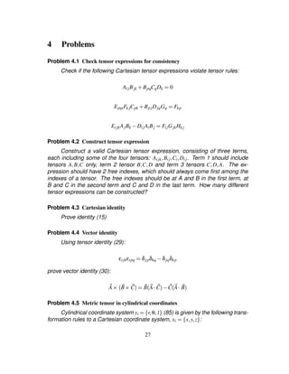
Preface
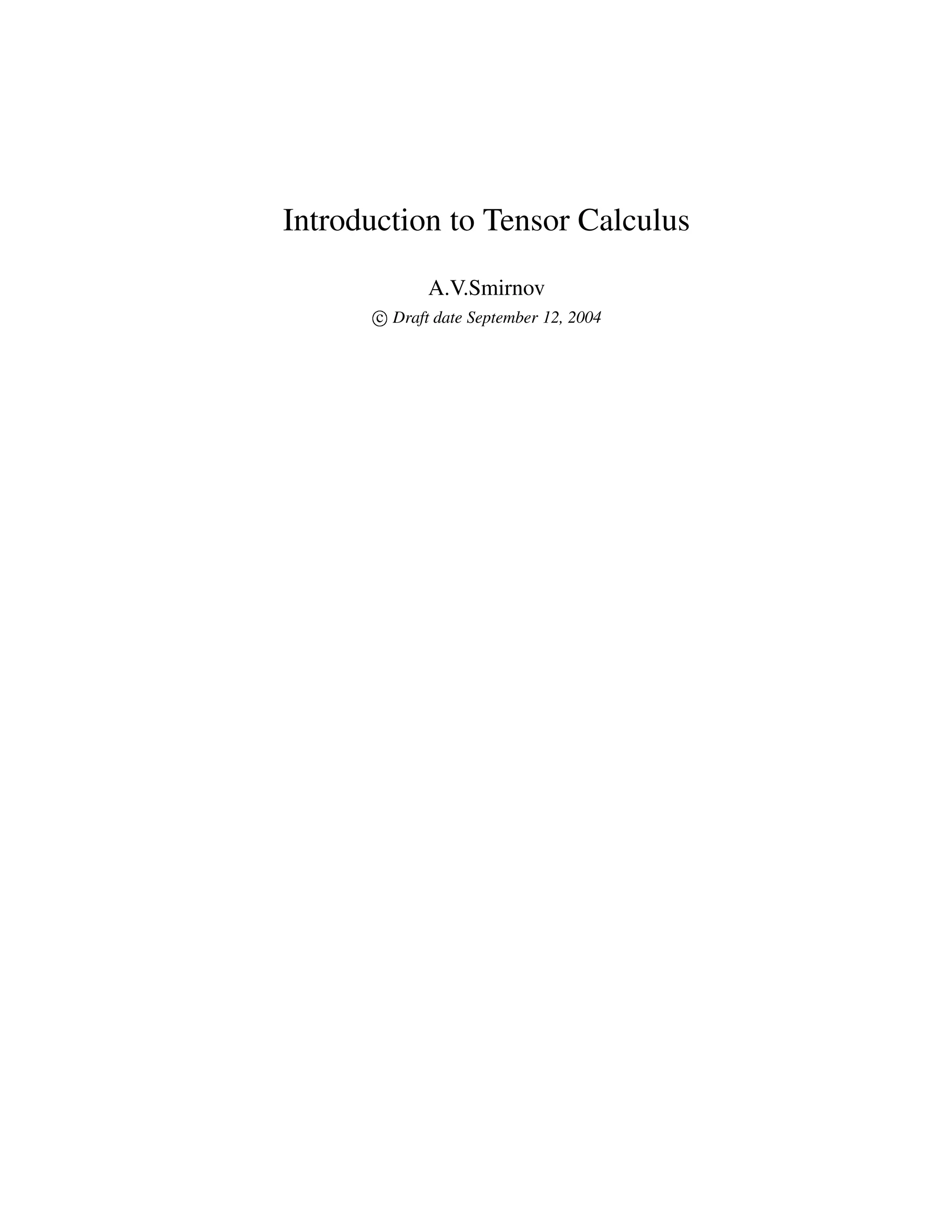
This material offers a short introduction to tensor calculus. It is directed toward
students of continuum mechanics and engineers. The emphasis is made on ten-
sor notation and invariant forms. A knowledge of calculus is assumed. A more
complete coverage of tensor calculus can be found in [1, 2].
Nomenclature
A ¡ B A is deﬁned as B, or A is equivalent to B
AiBi ¡ ∑3
i AiBi. Note: AiBi ¢ AjBj
˙A partial derivative over time: ∂A
∂t
A£i partial derivative over xi: ∂A
∂xi
V control volume
t time
xi i-th component of a coordinate (i=0,1,2), or xi ¡¥¤ x¦u¦z§
RHS Right-hand-side
LHS Left-hand-side
PDE Partial differential equation
.. Continued list of items
3

There are two aspects of tensors that are of practical and fundamental im-
portance: tensor notation and tensor invariance. Tensor notation is of great prac-
tical importance, since it simplifies handling of complex equation systems. The
idea of tensor invariance is of both practical and fundamental importance, since it
provides a powerful apparatus to describe non-Euclidean spaces in general and
curvilinear coordinate systems in particular.
A definition of a tensor is given in Section 1. Section 2 deals with an im-
portant class of Cartesian tensors, and describes the rules of tensor notation.
Section 3 provides a brief introduction to general curvilinear coordinates, invari-
ant forms and the rules of covariant differentiation.
1 Coordinates and Tensors
Consider a space of real numbers of dimension n, Rn, and a single real time,
t. Continuum properties in this space can be described by arrays of different
dimensions, m, such as scalars (m ¢ 0), vectors (m ¢ 1), matrices (m ¢ 2), and
general multi-dimensional arrays. In this space we shall introduce a coordinate
system, ¤ xi§ i¨ 1©©n, as a way of assigning n real numbers1 for every point of space
There can be a variety of possible coordinate systems. A general transformation
rule between the coordinate systems is
˜xi
¢ ˜xi x1 xn (1)
Consider a small displacement dxi. Then it can be transformed from coordi-
nate system xi to a new coordinate system ˜xi using the partial differentiation rules
applied to (1):
d ˜xi
¢ ∂ ˜xi
∂xj
dxj
(2)
This transformation rule2 can be generalized to a set of vectors that we shall call
contravariant vectors:
Ãi
¢ ∂˜xi
∂xj
Aj
(3)
1
Super-indexes denote components of a vector (i 1n) and not the power exponent, for the reason
explained later (Definition 1.1)
2The repeated indexes imply summation (See. Proposition 21)
4

That is, a contravariant vector is defined as a vector which transforms to a new
coordinate system according to (3). We can also introduce the transformation
matrix as:
ai
j ¡ ∂ ˜xi
∂xj
(4)
With which (3) can be rewritten as:
Ai
¢ ai
jAj
(5)
Transformation rule (3) will not apply to all the vectors in our space. For
example, a partial derivative ∂ ∂xi will transform as:
∂
∂ ˜xi ¢ ∂
∂ ˜xi
∂xj
∂xj ¢ ∂xj
∂ ˜xi
∂
∂xj
(6)
that is, the transformation coefficients are the other way up compared to (2). Now
we can generalize this transformation rule, so that each vector that transforms
according to (6) will be called a Covariant vector:
Ãi ¢ ∂xj
∂˜xi
Aj (7)
This provides the reason for using lower and upper indexes in a general
tensor notation.
Definition 1.1 Tensor
Tensor of order m is a set of nm numbers identified by m integer indexes. For
example, a 3rd order tensor A can be denoted as Aijk and an m-order tensor can
be denoted as Ai1 ©©im. Each index of a tensor changes between 1 and n. For ex-
ample, in a 3-dimensional space (n=3) a second order tensor will be represented
by 32
¢ 9 components.
Each index of a tensor should comply to one of the two transformation rules:
(3) or (7). An index that complies to the rule (7) is called a covariant index and is
denoted as a sub-index, and an index complying to the transformation rule (3) is
called a contravariant index and is denoted as a super-index.
Each index of a tensor can be covariant or a contravariant, thus tensor Ak
ij
is a 2-covariant, 1-contravariant tensor of third order.
5

From this relation and the independence of coordinates (9) it follows that ai
jb
j
k ¢
bi
ja
j
k ¢ δik, namely:
ai
jb
j
k ¢ ∂ ˜xi
∂xj
∂xj
∂ ˜xk
¢ ∂xj
∂xj
∂ ˜xi
∂ ˜xk ¢ ∂ ˜xi
∂ ˜xk ¢ δik (13)
2 Cartesian Tensors
Cartesian tensors are a sub-set of general tensors for which the transformation
matrix (4) satisfies the following relation:
ak
i ak
j ¢ ∂ ˜xk
∂xi
∂ ˜xk
∂xj ¢ δij (14)
For Cartesian tensors we have
∂ ˜xi
∂xk ¢ ∂xk
∂ ˜xi
(15)
(see Problem 4.3), which means that both (5) and (6) are transformed with the
same matrix ai
k. This in turn means that the difference between the covariant and
contravariant indexes vanishes for the Cartesian tensors. Considering this we
shall only use the sub-indexes whenever we deal with Cartesian tensors.
2.1 Tensor Notation
Tensor notation simplifies writing complex equations involving multi-dimensional
objects. This notation is based on a set of tensor rules. The rules introduced in
this section represent a complete set of rules for Cartesian tensors and will be
extended in the case of general tensors (Sec.3). The importance of tensor rules
is given by the following general remark:
Remark 2.1 Tensor rules Tensor rules guarantee that if an expression follows
these rules it represents a tensor according to Definition 1.1.
7

Tensors are usually functions of space and time:
Ai1 ©©im ¢ Ai1 ©©im
x1 xn
¦t
which defines a tensor field, i.e. for every point xi and time t there are a set of mn
nubers Ai1 ©©im.
Remark 1.2 Tensor character of coordinate vectors
Note, that the coordinates xi are not tensors, since generally, they are not
transformed as (5). Transformation law for the coordinates is actually given by (1).
Nevertheless, we shall use the upper (contravariant) indexes for the coordinates.
Definition 1.3 Kronecker delta tensor
Second order delta tensor, δij is defined as
i ¢ j ! δij ¢ 1
i ¢ j ! δij ¢ 0 (8)
From this definition and since coordinates xi are independent of each other
it follows that:
∂xi
∂xj ¢ δij (9)
Corollary 1.4 Delta product
From the definition (1.3) and the summation convention (21), follows that
δijAj ¢ Ai (10)
Assume that there exists the transformation inverse to (5), which we call bi
j:
dxi
¢ bi
jd ˜xj
(11)
Then by analogy to (4) bi
j can be defined as:
bi
j ¢ ∂xi
∂ ˜xj
(12)
6

Thus, following tensor rules, one can build tensor expressions that will pre-
serve tensor properties of coordinate transformations (Definition 1.1) and coordi-
nate invariance (Section 3).
Tensor rules are based on the following definitions and propositions.
Definition 2.2 Tensor terms
A tensor term is a product of tensors.
For example:
AijkBjkCpqEqFp (16)
Definition 2.3 Tensor expression
Tensor expression is a sum of tensor terms. For example:
AijkBjk # CiDpqEqFp (17)
Generally the terms in the expression may come with plus or minus sign.
Proposition 2.4 Allowed operations
The only allowed algebraic operations in tensor expressions are the addi-
tion, subtraction and multiplication. Divisions are only allowed for constants, like
1 C. If a tensor index appears in a denominator, such term should be redefined,
so as not to have tensor indexes in a denominator. For example, 1 Ai should be
redefined as: Bi ¡ 1 Ai.
Definition 2.5 Tensor equality
Tensor equality is an equality of two tensor expressions.
For example:
AijBj ¢ CikpDkEp # EjCjkiBk (18)
8

Deﬁnition 2.6 Free indexes
A free index is any index that occurs only once in a tensor term. For exam-
ple, index i is a free index in the term (16).
Proposition 2.7 Free index restriction
Every term in a tensor equality should have the same set of free indexes.
For example, if index i is a free index in any term of tensor equality, such as
(18), it should be the free index in all other terms. For example
AijBj ¢ CjDj
is not a valid tensor equality since index i is a free index in the term on the
RHS but not in the LHS.
Deﬁnition 2.8 Rank of a term
A rank of a tensor term is equal to the number of its free indexes.
For example, the rank of the term AijkBjCk is equal to 1.
It follows from (2.7) that ranks of all the terms in a valid tensor expression
should be the same. Note, that the difference between the order and the rank is
that the order is equal to the number of indexes of a tensor, and the rank is equal
to the number of free indexes in a tensor term.
Proposition 2.9 Renaming of free indexes
Any free index in a tensor expression can be named by any symbol as long
as this symbol does not already occur in the tensor expression.
For example, the equality
AijBj ¢ CiDjEj (19)
is equivalent to
Ak jBj ¢ CkDjEj (20)
Here we replaced the free index i with k.
9

Definition 2.10 Dummy indexes
A dummy index is any index that occurs twice in a tensor term.
For example, indexes j¦k¦ p¦q in (16) are dummy indexes.
Proposition 2.11 Summation rule
Any dummy index implies summation, i.e.
AiBi ¢
n
∑
i
AiBi (21)
Proposition 2.12 Summation rule exception If there should be no summation
over the repeated indices, it can be indicated by enclosing such indices in paren-
theses.
For example, expression:
C$i%A$i%Bj ¢ Dij
does not imply summation over i.
Corollary 2.13 Scalar product
A scalar product notation from vector algebra: A B is expressed in tensor
notation as AiBi.
The scalar product operation is also called a contraction of indexes.
Proposition 2.14 Dummy index restriction
No index can occur more than twice in any tensor term.
Remark 2.15 Repeated indexes
In case if an index occurs more than twice in a term this term should be
redefined so as not to contain more than two occurrences of the same index. For
example, term AikBjkCk should be rewritten as AikDjk, where Djk is defined as
Djk ¡ Bj$k%C$k% with no summation over k in the last term.
10

Proposition 2.16 Renaming of dummy indexes
Any dummy index in a tensor term can be renamed to any symbol as long
as this symbol does not already occur in this term.
For example, term AiBi is equivalent to AjBj, and so are terms AijkBjCk and
AipqBpCq.
Remark 2.17 Renaming rules
Note that while the dummy index renaming rule (2.16) is applied to each
tensor term separately, the free index naming rule (2.9) should apply to the whole
tensor expression. For example, the equality (19) above
AijBj ¢ CiDjEj
can also be rewritten as
AkpBp ¢ CkDjEj (22)
without changing its meaning.
(See Problem 4.1).
Deﬁnition 2.18 Permutation tensor
The components of a third order permutation tensor εijk are deﬁned to be
equal to 0 when any index is equal to any other index; equal to 1 when the set of
indexes can be obtained by cyclic permutation of 123; and -1 when the indexes
can be obtained by cyclic permutation from 132. In a mathematical language it
can be expressed as:
i ¢ j ' i ¢ k ' j ¢ k ! εijk ¢ 0
i jk ( PG123 ! εijk ¢ 1
i jk ( PG132 ! εijk ¢0) 1 (23)
where PGabc is a permutation group of a triple of indexes abc, i.e. PGabc ¢¤ abc¦bca¦cab§ . For example, the permutation group of 123 will consist of three
combinations: 123, 231 and 312, and the permutation group of 123 consists of
132, 321 and 213.
11

Corollary 2.19 Permutation of the permutation tensor indexes
From the deﬁnition of the permutation tensor it follows that the permutation
of any of its two indexes changes its sign:
εijk ¢1) εik j (24)
A tensor with this property is called skew-symmetric.
Corollary 2.20 Vector product
A vector product (cross-product) of two vectors in vector notation is ex-
pressed as
2A ¢ 2B 3 2C (25)
which in tensor notation can be expressed as
Ai ¢ εijkBjCk (26)
Remark 2.21 Cross product
Tensor expression (26) is more accurate than its vector counterpart (25),
since it explicitly shows how to compute each component of a vector product.
Theorem 2.22 Symmetric identity
If Aij is a symmetric tensor, then the following identity is true:
εijkAjk ¢ 0 (27)
Proof:
From the symmetry of Aij we have:
εijkAjk ¢ εijkAk j (28)
Let’s rename index j into k and k into j in the RHS of this expression, according
to rule (2.16):
εijkAk j ¢ εik jAjk
12

Using (24) we ﬁnally obtain:
εik jAjk ¢1) εijkAjk
Comparing the RHS of this expression to the LHS of (28) we have:
εijkAjk ¢1) εijkAjk
from which we conclude that (27) is true.
Theorem 2.23 Tensor identity
The following tensor identity is true:
εijkεipq ¢ δjpδkq ) δjqδkp (29)
Proof
This identity can be proved by examining the components of equality (29)
component-by-component.
Corollary 2.24 Vector identity
Using the tensor identity (29) it is possible to prove the following important
vector identity:
2A 3 2B 3 2C ¢ 2B 2A 2C ) 2C 2A 2B (30)
See Problem 4.4.
2.2 Tensor Derivatives
For Cartesian tensors derivatives introduce the following notation.
Deﬁnition 2.25 Time derivative of a tensor
A partial derivative of a tensor over time is designated as
˙A ¡ ∂A
∂t
13

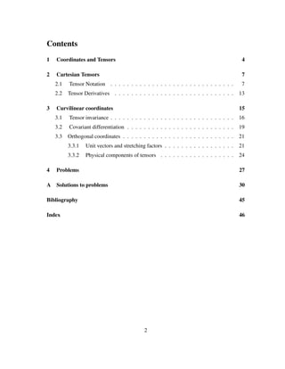
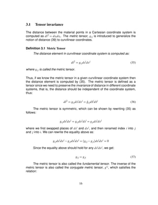
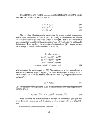
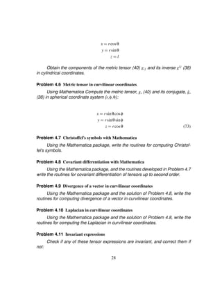
Definition 2.26 Spatial derivative of a tensor
A partial derivative of a tensor A over one or its spacial components is de-
noted as A£i:
A£i ¡ ∂A
∂xi
(31)
that is, the index of the spatial component that the derivation is done over is
delimited by a comma (’,’) from other indexes. For example, Aij£k is a derivative of
a second order tensor Aij.
Definition 2.27 Nabla
Nabla operator acting on a tensor A is defined as
∇iA ¡ A£i (32)
Even though the notation in (31) is sufficient to define the derivative, In some
instances it is convenient to introduce the nabla operator as defined above.
Remark 2.28 Tensor derivative
In a more general context of non-Cartesian tensors the coordinate indepen-
dent derivative will have a different form from (31). See the chapter on covariant
differentiation in [1].
Remark 2.29 Rank of a tensor derivative
The derivative of a zero order tensor (scalar) as given by (31) forms a first
order tensor (vector). Generally, the derivative of an m-order tensor forms an m# 1
order tensor. However, if the derivation index is a dummy index, then the rank of
the derivative will be lower than that of the original tensor. For example, the rank
of the derivative Aij£j is one, since there is only one free index in this term.
Remark 2.30 Gradient
Expression (31) represents a gradient, which in a vector notation is ∇A:
∇A )54 A£i
14

Corollary 2.31 Derivative of a coordinate
From (9) it follows that:
xi£j ¢ δij (33)
In particular, the following identity is true:
xi£i ¢ x1£1 # x2£2 # x3£3 ¢ 1 # 1 # 1 ¢ 3 (34)
Remark 2.32 Divergence operator
A divergence operator in a vector notation is represented in a tensor notation
as Ai£i:
∇ 2A )54 Ai£i
Remark 2.33 Laplace operator
The Laplace operator in vector notation is represented in tensor notation as
A£ii:
∆A )54 A£ii
Remark 2.34 Tensor notation
Examples (2.30), (2.32) and (2.33) clearly show that tensor notation is more
concise and accurate than vector notation, since it explicitly shows how each
component should be computed. It is also more general since it covers cases
that don’t have representation in vector notation, for example: Aik£k j.
3 Curvilinear coordinates
In this section 3 we introduce the idea of tensor invariance and introduce the rules
for constructing invariant forms.
3
In this section we reinstall the difference between covariant and contravariant indexes.
15

3.1 Tensor invariance
The distance between the material points in a Cartesian coordinate system is
computed as dl2
¢ dxidxi. The metric tensor, gij is introduced to generalize the
notion of distance (39) to curvilinear coordinates.
Definition 3.1 Metric Tensor
The distance element in curvilinear coordinate system is computed as:
dl2
¢ gijdxi
dxj
(35)
where gij is called the metric tensor.
Thus, if we know the metric tensor in a given curvilinear coordinate system then
the distance element is computed by (35). The metric tensor is defined as a
tensor since we need to preserve the invariance of distance in different coordinate
systems, that is, the distance should be independent of the coordinate system,
thus:
dl2
¢ gijdxi
dxj
¢ ˜gijd ˜xi
d ˜xj
(36)
The metric tensor is symmetric, which can be shown by rewriting (35) as
follows:
gijdxi
dxj
¢ gijdxj
dxi
¢ gjidxi
dxj
where we first swapped places of dxi and dxj, and then renamed index i into j
and j into i. We can rewrite the equality above as:
gijdxi
dxj
) gjidxi
dxj
¢ gij ) gji
dxi
dxj
¢ 0
Since the equality above should hold for any dxidxj, we get:
gij ¢ gji (37)
The metric tensor is also called the fundamental tensor. The inverse of the
metric tensor is also called the conjugate metric tensor, gij, which satisfies the
relation:
16

gik
gk j ¢ δij (38)
Let xi be a Cartesian coordinate system, and ˜xj - the new curvilinear coordi-
nate system. Both systems are related by transformation rules (5) and (11). Then
from (36) we get:
dl2
¢ dxi
dxi
¢ ∂xi
∂˜xj
d ˜xj ∂xi
∂˜xk
d ˜xk
¢ ∂xi
∂˜xj
∂xi
∂˜xk
d ˜xj
d ˜xk
(39)
When we transform from a Cartesian to curvilinear coordinates the metric
tensor in curvilinear coordinate system, ˜gij can be determined by comparing re-
lations (39) and (35):
˜gij ¢ ∂xk
∂ ˜xi
∂xk
∂ ˜xj
(40)
Using (38) we can also find its inverse as:
˜gij
¢ ∂˜xi
∂xk
∂˜xj
∂xk
(41)
Using these expression one can compute gij and gij in various curvilinear coordi-
nate systems (see Problem 4.6).
Definition 3.2 Conjugate tensors
For each index of a tensor we introduce the conjugate tensor where this
index is transfered to its counterpart (covariant/contravariant) using the relations:
Ai
¢ gij
Aj (42)
Ai ¢ gijAj
(43)
Conjugate tensor is also called the associate tensor. Relations (42), (43)
are also called as operations of raising/lowering of indexes.
Remark 3.3 Tensor invariance
Since the transformation rules defined by (1.1) have a simple multiplicative
character, any tensor expression should retain it’s original form under transforma-
tion into a new coordinate system. Thus if an expression is given in a tensor form
it will be invariant under coordinate transformations.
17

Not all the expressions constructed from tensor terms in curvilinear coordi-
nates will be tensors themselves. For example, if vectors Ai and Bi are tensors,
then AiBi is not generally a tensor4. However, if we consider the same operation
on a contravariant tensor Ai and a covariant tenso Bi then the product will form an
invariant:
¯Ai ¯Bi ¢ Ai
Bi (44)
Thus in curvilinear coordinates we have to refine the definition of the scalar
product (Corollary 2.13) or the index contraction operation to make it invariant
(Problem 4.12).
Definition 3.4 Invariant Scalar Product
The invariant form of the scalar product between two covariant vectors Ai
and Bi is gijAiBj. Similarly, the invariant form of a scalar product between two
contravariant vectors Ai and Bi is gijAiBj, where gij is the metric tensor (40) and
gij is its conjugate (38).
Corollary 3.5 Two forms of a scalar product
According to (42), (43) the scalar product can be represented by two invari-
ant forms: AiBi and AiBi. It can be easily shown that these two forms have the
same values (see Problem 4.12).
Corollary 3.6 Rules of invariant expressions
To build invariant tensor expressions we add two more rules to Cartesian
tensor rules outlined in Section 2.1:
1. Each free index should keep its vertical position in every term, i.e. if the
index is covariant in one term it should be covariant in every other term, and
vise versa.
2. Every pair of dummy indexes should be complementary, that is one should
be covariant, and another contravariant.
For example, a Cartesian formulation of a momentum equation for an in-
compressible viscous fluid is
˙ui # ukui£k ¢0) P£i
ρ
# ντik£k
4For Cartesian tensors any product of tensors will always be a tensor, but this is not so for general tensors
18

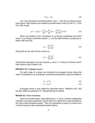
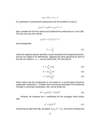
The invariant form of this equation is:
˙ui # uk
ui£k ¢0) P£i
ρ
# ντk
i£k (45)
where the rising of indexes was done using relation (42): uk
¢ gk juj, and τk
i ¢gk jτij.
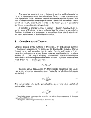
3.2 Covariant differentiation
A simple scalar value, S, is invariant under coordinate transformations. A partial
derivative of an invariant is a ﬁrst order covariant tensor (vector):
Ai
¢ S£i ¢ ∂S
∂xi
However, a partial derivative of a tensor of the order one and greater is not
generally an invariant under coordinate transformations of type (7) and (3).
In curvilinear coordinate system we should use more complex differentiation
rules to preserve the invariance of the derivative. These rules are called the rules
of covariant differentiation and they guarantee that the derivative itself is a tensor.
According to these rules the derivatives for covariant and contravariant indices
will be slightly different. They are expressed as follows:
Ai£j ¡ ∂Ai
∂xj )
6 k
ij 7 Ak (46)
Ai
£j ¡ ∂Ai
∂xj #
6 i
k j 7 Ak
(47)
where the contstruct
6 k
ij 7 is deﬁned as
6 k
ij 7 ¢ 1
2
gkl 8 ∂gil
∂xj # ∂gjl
∂xi ) ∂gij
∂xl 9
and is also known in tensor calculus as Christoffel’s symbol of the second kind
[1]. Tensor gij represents the inverse of the metric tensor gij (38). As can be seen
differentiation of a single component of a vector will involve all other components
of this vector.
19

In differentiating higher order tensors each index should be treated inde-
pendently. Thus differentiating a second order tensor, Aij, should be performed
as:
Aij£k ¢ ∂Aij
∂xk ) ¤ m
ik § Amj ) ¤ m
jk § Aim
and as can be seen also involves all the components of this tensor. Likewise for
the contravariant second order tensor Aij we have:
A
ij
£k ¢ ∂Aij
∂xk # ¤ i
mk § Amj
# ¤ j
mk § Aim
(48)
And for a general n-covariant, m-contravariant tensor we have:
A
j1 ©©jm
i1 ©©in £p ¢ ∂
∂xp
A
j1 ©©jm
i1 ©©in £k
# ¤ j1
qp § A
qj2 ©©jm
i1 ©©in # @A # ¤ jm
qp§ A
j1 ©©jmB 1q
i1 ©©in
# ¤ q
i1 p§ A
j1 ©©jm
qi2 ©©in # @@ # ¤ q
in p § A
j1 ©©jm
i1 ©©inB 1q (49)
Despite their seeming complexity, the relations of covariant differentiation
can be easily implemented algorithmically and used in numerical solutions on
arbitrary curved computational grids (Problem 4.8).
Remark 3.7 Rules of invariant expressions
As was pointed out in Corollary 3.6, the rules to build invariant expressions
involve raising or lowering indexes (42), (43). However, since we did not intro-
duce the notation for contravariant derivative, the only way to raise the index of a
covariant derivative, say A£i, it to use the relation (42) directly, that is: gijA£j.
For example, we can re-formulate the momentum equation (45) in terms of
contravariant free index i as:
˙ui
# uk
ui
£k ¢1) gikP£k
ρ
# ντik
£k (50)
where the index of the pressure term was raised by means of (42).
Using the invariance of the scalar product one can construct two important
differential operators in curvilinear coordinates: divergence of a vector divA ¡ Ai
£i
(51) and Laplacian, ∆A ¡ gikA£ki (55).
20

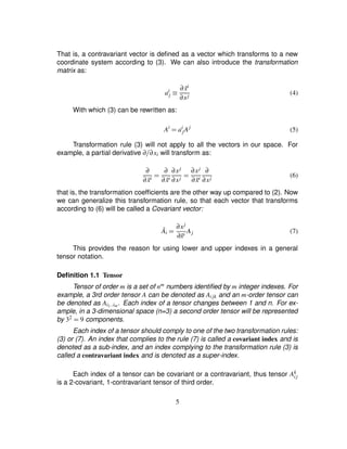
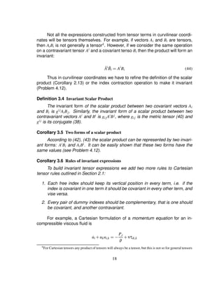
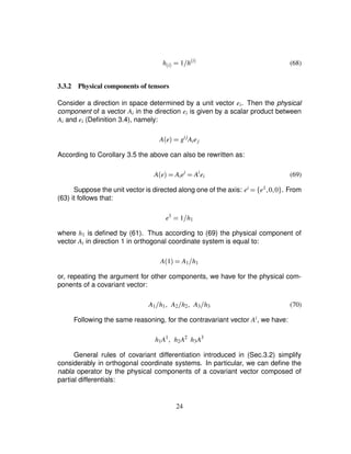
Definition 3.8 Divergence
Divergence of a vector is defined as Ai
£i:
divA ¡ Ai
£i (51)
From this definition and the rule of covariant differentiation (47) we have:
Ai
£i ¢ ∂Ai
∂xi # ¤ i
ki§ Ak
(52)
this can be shown [2] to be equal to:
Ai
£i ¢ ∂Ai
∂xi # 8 1
C g
∂
∂xi
C g9 Ai
¢ 1
C g
∂
∂xi D C gAiE (53)
where g is the determinant of the metric tensor gij.
The divergence of a covariant vector Ai is defined as a divergence of its
conjugate contravariant tensor (42):
Ai
£i ¢ gij
Aj£i (54)
Definition 3.9 Laplacian
A Laplace operator or a Laplacian of a scalar A is defined as
∆A ¡ gik
A£ki (55)
The definitions (3.8), (3.9) of differential operators are invariant under coor-
dinate transformations. They can be programmed using a symbolic manipulation
packages and used to derive expressions in different curvilinear coordinate sys-
tems (Problem 4.9).
3.3 Orthogonal coordinates
3.3.1 Unit vectors and stretching factors
The coordinate system is orthogonal if the tangential vectors to coordinate lines
are orthogonal at every point.
21

Consider three unit vectors, ai¦bi ¦ci, each directed along one of the coordi-
nate axis (tangential unit vectors), that is:
ai
¢ ¤ a1
¦0¦0§ (56)
bi
¢ ¤ 0¦b2
¦0§ (57)
ci
¢ ¤ 0¦0¦c3
§ (58)
The condition of orthogonality means that the scalar product between any
two of these unit vectors should be zero. According to the definition of a scalar
product (Definition 3.4) it should be written in form (44), that is, a scalar product
between vectors ai and bi can be written as: aibi or aibi. Let’s use the first form for
definiteness. Then, applying the operation of rising indexes (42), we can express
the scalar product in contravariant components only:
0 ¢ ai
bi ¢ gijai
bj
¢
g11a1
0 # g12a1
b2
# g1300
g21a2
b1
# g220b2
# g2300
g31a3
0 # g320b2
# g3300
¢ g12 # g21
a1
b2
¢ 2g12a1
b2
¢ 0 (59)
where we used the symmetry of gij, (37). Since vectors a1 and b2 were chosen to
be non-zero, we have: g12 ¢ 0. Applying the same reasoning for scalar products of
other vectors, we conclude that the metric tensor has only diagonal components
non-zero5:
gij ¢ δijg$ii% (60)
Let’s introduce stretching factors, hi, as the square roots of these diagonal com-
ponents of gij:
h1 ¡ g11
1F2
; h2 ¡ g22
1F2
; h3 ¡ g33
1F2
; (61)
Now, consider the scalar product of each of the unit vectors (56)-(58) with
itself. Since all vectors are unit, the scalar product of each with itself should be
one:
5We use parenthesis to preclude summation (Proposition 2.12)
22

ai
ai ¢ bi
bi ¢ ci
ci ¢ 1
Or, expressed in contravariant components only the condition of unity is:
gijai
aj
¢ gijbi
bj
¢ gijci
cj
¢ 1
Now, consider the first term above and substitute the components of a from (56).
The only non-zero term will be:
g11a1
a1
¢ h1
2 a1 2
¢ 1
and consequently:
a1
¢HG 1
h1
(62)
where the negative solution identifies a vector directed into the opposite direction,
and we can neglect it for definiteness. Applying the same reasoning for each of
the tree unit vectors ai ¦bi¦ci, we can rewrite (56), (57) and (58) as:
ai
¢ ¤ 1
h1
¦0¦0§ (63)
bi
¢ ¤ 0¦ 1
h2
¦0§ (64)
ci
¢ ¤ 0¦0¦ 1
h3
§ (65)
which means that the components of unit vectors in a curved space should be
scaled with coefficients hi. It follows from this that the expression for the element
of length in curvilinear coordinates, (35), can be written as:
dl2
¢ gijd ˜xi
d ˜xj
¢ h2
i
d ˜xi 2
(66)
Similarly, we introduce the hi coefficients for the conjugate metric tensor
(38):
gij
¢ δij
h
$i % 2
(67)
Combining the latter with (38), we obtain: δijh$i%h
$i% ¢ δij, from which it follows that
23

h$i% ¢ 1 h
$i% (68)
3.3.2 Physical components of tensors
Consider a direction in space determined by a unit vector ei. Then the physical
component of a vector Ai in the direction ei is given by a scalar product between
Ai and ei (Definition 3.4), namely:
Ae ¢ gij
Aiej
According to Corollary 3.5 the above can also be rewritten as:
Ae ¢ Aiei
¢ Ai
ei (69)
Suppose the unit vector is directed along one of the axis: ei
¢ ¤ e1 ¦0¦0§ . From
(63) it follows that:
e1
¢ 1 h1
where h1 is defined by (61). Thus according to (69) the physical component of
vector Ai in direction 1 in orthogonal coordinate system is equal to:
A1 ¢ A1 h1
or, repeating the argument for other components, we have for the physical com-
ponents of a covariant vector:
A1 h1 ¦ A2 h2 ¦ A3 h3 (70)
Following the same reasoning, for the contravariant vector Ai, we have:
h1A1
¦ h2A2
h3A3
General rules of covariant differentiation introduced in (Sec.3.2) simplify
considerably in orthogonal coordinate systems. In particular, we can define the
nabla operator by the physical components of a covariant vector composed of
partial differentials:
24

∇i ¢ 1
h$i%
∂
∂xi
(71)
where the parentheses indicate that there’s no summation with respect to index i.
In orthogonal coordinate system the general expressions for divergence (53)
and Laplacian (55)) operators can be expressed in terms of stretching factors only
[3]:
Ai
£i ¢ 1
H
∂
∂xi I
H
h$i% AiP (72)
∆A ¢ 1
H
∂
∂xi I
H
h$i%
A
∂xi
P
H ¡ n
∏
i¨ 1
hi
Important examples of orthogonal coordinate systems are spherical and cylindri-
cal coordinate systems. Consider the example of a cylindrical coordinate system:
xi ¢ ¤ x1 ¦x2¦x3§ and ˜xi ¢ ¤ r¦θ¦ l§ :
x1 ¢ rcosθ
x2 ¢ rsinθ
x3 ¢ l
According to (40) only few components of the metric tensor will survive
(Problem 4.5). Then we can compute nabla, divergence and Laplacian oper-
ators according to (71), (52) and (55), or using simpliﬁed relations (72)-(73):
∇ ¢ 8 ∂
∂r
¦ 1
r
∂
∂θ
¦ ∂
∂z9
divA ¢ ∂A1
∂ ˜x1 # 1
˜x1
∂A2
∂ ˜x2 # ∂A3
∂ ˜x3 # 1
˜x1
A1
¢ ∂Ar
∂r
# 1
r
∂Aθ
∂θ
# ∂Az
∂z
# 1
r
Ar
Note, that instead of using the contravariant components as implied by the gen-
eral deﬁnition of the divergence operator (51) we are using the covariant compo-
nents as dictated by relation (70). The expression of the Laplacian becomes:
25

∆A ¢ ∂2 A
∂ ˜x1
2 # 1
˜x2
1
∂2 A
∂ ˜x2
2 # ∂2 A
∂ ˜x3
2 # 1
˜x1
∂A
∂ ˜x1
¢ ∂2A
∂r 2 # 1
r2
∂2A
∂θ 2 # ∂2A
∂z 2 # 1
r
∂A
∂r
(see Problems 4.9,4.10).
The advantages of the tensor approach are that it can be used for any type
of curvilinear coordinate transformations, not necessarily analytically deﬁned, like
cylindrical (85) or spherical. Another advantage is that the equations above can
be easily produced automatically using symbolic manipulation packages, such
as Mathematica (wolfram.com) (Problems 4.6,4.7,4.9). For further reading see
[1, 2].
26

4 Problems
Problem 4.1 Check tensor expressions for consistency
Check if the following Cartesian tensor expressions violate tensor rules:
AijBjk # BpqCqDk ¢ 0
EpqiFk jCpk # BpjDjqGq ¢ Fkp
EijkAjBk ) DijAiBj ¢ FijGjkHk j
Problem 4.2 Construct tensor expression
Construct a valid Cartesian tensor expression, consisting of three terms,
each including some of the four tensors: Aijk ¦Bij ¦Ci ¦Dij. Term 1 should include
tensors A¦B¦C only, term 2 tensor B¦C¦D and term 3 tensors C¦D¦A. The ex-
pression should have 2 free indexes, which should always come ﬁrst among the
indexes of a tensor. The free indexes should be at A and B in the ﬁrst term, at
B and C in the second term and C and D in the last term. How many different
tensor expressions can be constructed?
Problem 4.3 Cartesian identity
Prove identity (15)
Problem 4.4 Vector identity
Using tensor identity (29):
εijkεipq ¢ δjpδkq ) δjqδkp
prove vector identity (30):
2A 3 2B 3 2C ¢ 2B 2A 2C ) 2C 2A 2B
Problem 4.5 Metric tensor in cylindrical coordinates
Cylindrical coordinate system yi ¢ ¤ r¦θ¦ l§ (85) is given by the following trans-
formation rules to a Cartesian coordinate system, xi ¢ ¤ x¦y¦z§ :
27

x ¢ rcosθ
y ¢ rsinθ
z ¢ l
Obtain the components of the metric tensor (40) gij and its inverse gij (38)
in cylindrical coordinates.
Problem 4.6 Metric tensor in curvilinear coordinates
Using Mathematica Compute the metric tensor, g, (40) and its conjugate, ˆg,
(38) in spherical coordinate system (r¦φ¦θ):
x ¢ rsinθcosφ
y ¢ rsinθsinφ
z ¢ rcosθ (73)
Problem 4.7 Christoffel’s symbols with Mathematica
Using the Mathematica package, write the routines for computing Christof-
fel’s symbols.
Problem 4.8 Covariant differentiation with Mathematica
Using the Mathematica package, and the routines developed in Problem 4.7
write the routines for covariant differentiation of tensors up to second order.
Problem 4.9 Divergence of a vector in curvilinear coordinates
Using the Mathematica package and the solution of Problem 4.8, write the
routines for computing divergence of a vector in curvilinear coordinates.
Problem 4.10 Laplacian in curvilinear coordinates
routines for computing the Laplacian in curvilinear coordinates.
Problem 4.11 Invariant expressions
Check if any of these tensor expressions are invariant, and correct them if
not:
28

AiBi
jkC
j
t£k ¢ Dt (74)
A
ij
jkBipqCkq
) Fk jGk
pH j
¢ Hk
A
jq
k jCti
Bpit£q (75)
Ei
Bi
kp # D
p
kqC
j
jq ¢ DkiGp£i (76)
Problem 4.12 Contraction invariance
Prove that AiBi is an invariant and AiBi is not.
29

A Solutions to problems
Problem 4.1: Check tensor expressions
Check if the following Cartesian tensor expressions violate tensor rules:
AijBjk # BpqCqDk ¢ 0
Answer: term (1): ik = free, term (2): pk=free
EpqiFk jCpk # BpjDjqGq ¢ Fkp
Answer: (1): ijq=free (2): p=free (3): kp=free
EijkAjBk ) DijAiBj ¢ FijGjkHk j
Answer: (1): i=free (2): none, (3): i=free, j = tripple occurrence
Problem 4.2: Construct tensor expression
Construct a valid Cartesian tensor expression, consisting of three terms,
each including some of the four tensors: Aijk ¦Bij ¦Ci ¦Dij. Term 1 should include
tensors A¦B¦C only, term 2 tensor B¦C¦D and term 3 tensors C¦D¦A. The ex-
pression should have 2 free indexes, which should always come ﬁrst among the
indexes of a tensor. The free indexes should be at A and B in the ﬁrst term, at
B and C in the second term and C and D in the last term. How many different
tensor expressions can be constructed?
Solution
One possibility is:
AipkBjkCp # BiqCpCjDpq # CiDjpApqq ¢ 0
Since there are four locations for dummy indexes in each term, there could
be three different combinations of dummies in each term. Thus, the total number
of different expression is 33
¢ 27
30

Problem 4.3: Cartesian identity
Prove identity (15).
Proof
Integrating (5) in the case of constant transformation marix coefﬁcients, we
have:
˜xi
¢ ai
kxk
# bi
(77)
where the transformation matrix is given by (4):
ai
k ¡ ∂ ˜xi
∂xk
(78)
By the deﬁnition of the Cartesian coordinates (79) we have:
ak
i ak
j ¢ ∂ ˜xk
∂xi
∂ ˜xk
∂xj ¢ δij (79)
Let’s multiply the transformation rule (77) by ai
j. Then we get:
ai
j ˜xi
¢ ai
jai
kxk
# ai
jbi
¢ δjkxk
# ai
jbi
¢ xj
# ai
jbi
Differentiation this over ˜xi, we have:
ai
j ¢ ∂xj
∂˜xi
Now rename index j into k:
ai
k ¢ ∂xk
∂˜xi
Comparing this with (78), we have
∂˜xi
∂xj ¢ ∂xj
∂˜xi
which proves (15).
31

Problem 4.4: Tensor identity
Using the tensor identity:
εijkεipq ¢ δjpδkq ) δjqδkp (80)
prove the vector identity (30):
2A 3 2B 3 2C ¢ 2B 2A 2C ) 2C 2A 2B (81)
Proof
Applying (26) twice to the RHS of (81), we have:
2A 3 2B 3 2C
¢ εijkAjεkpqBpCq
¢ εijkεkpqAjBpCq
From (24) it follows that εijk ¢1) εik j ¢ εkij. Then we have:
εijkεkpqAjBpCq ¢ εkijεkpqAjBpCq (82)
Now rename the dummy indexes: k 4 i¦i 4 j¦ j 4 k, so that the expression
looks like one in (29):
εijkεipq
AkBpCq
¢ δjpδkq ) δjqδkp
AkBpCq
¢ δjpBpδkqAkCq ) δjqCqδkpAkBp (83)
Using (10), and since Aj ¢ Bj is the same as Ai ¢ Bi the latter can be rewrit-
ten as:
¢ BjAqCq ) CjApBp (84)
which is the same as
2B 2A 2C ) 2C 2A 2B
32

Problem 4.5: Metric tensor in cylindrical coordinates.
Cylindrical coordinate system ˜xi
¢ ¤ r¦θ¦ l§ (85) is given by the following trans-
formation rules to a Cartesian coordinate system, xi
¢ ¤ x¦y¦z§ :
x ¢ rcosθ
y ¢ rsinθ
z ¢ l
Obtain the components of the metric tensor (40) gij and its inverse gij (38)
in cylindrical coordinates.
Solution:
First compute the derivatives of xi
¢ ¤ x¦y¦z§ with respect to ˜xi
¢ ¤ r¦θ¦ l§ :
∂x1
∂˜x1 ¢ ∂x
∂r
¡ xr ¢ cosθ
∂x2
∂˜x1 ¢ ∂y
∂r
¡ yr ¢ sinθ
∂x1
∂˜x2 ¢ ∂x
∂θ
¡ xθ ¢0) rsinθ
∂x2
∂˜x2 ¢ ∂y
∂θ
¡ yθ ¢ rcosθ
∂x3
∂˜x3 ¢ ∂z
∂z
¡ zl ¢ 1 (85)
Then the components of the metric tensor are:
grr ¢ xrxr # yryr ¢ 1
gθθ ¢ xθ xθ # yθ yθ ¢ r2
gzz ¢ 1
grr
¢ 1
gθθ
¢ 1
r2
gzz
¢ 1
33

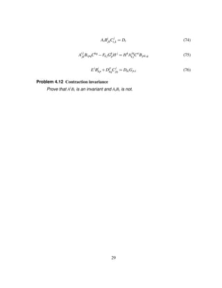
Problem 4.6: Metric tensor in curvilinear coordinates
Using Mathematica, write a procedure to compute metric tensor in curvilin-
ear coordinate system, and use it to obtain the components of metric tensor, g,
(40) and its conjugate, ˆg, (38) in spherical coordinate system (r¦φ¦θ):
x ¢ rsinθcosφ
y ¢ rsinθsinφ
z ¢ rcosθ (86)
Solution with Mathematica
NX = 3
(* Curvilinear cooridnate system *)
Y = Array[,NX] (* Spherical coordinate system *)
Y[[1]] = r; (* radius *)
Y[[2]] = th; (* angle theta *)
Y[[3]] = phi; (* angle phi *)
(* Cartesian coordinate system *)
X = Array[,NX]
X[[1]] = r Sin[th] Cos[phi];
X[[2]] = r Sin[th] Sin[phi];
X[[3]] = r Cos[th];
(* Compute the Jacobian: dXi/dYj *)
J = Array[,{NX,NX}]
Do[
J [[i,j]] = D[X[[i]],Y[[j]]],
{j,1,NX},{i,1,NX}
]
(* Covariant Metric tensor *)
g = Array[,{NX,NX}] (* covariant *)
Do[
g [[i,j]] = Sum[J[[k,i]] J[[k,j]],{k,NX}],
{j,1,NX},{i,1,NX}
34

];
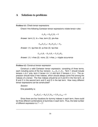
g=Simplify[g]
(* Contravariant metric tensor *)
g1 =Array[,{NX,NX}]
g1=Inverse[g]
With the result:
g ¢ ¤Q¤ 1¦0¦0§R¦A¤ 0¦r2
¦0§R¦A¤ 0¦0¦r2
sinθ2
§Q§
ˆg ¢ ¤Q¤ 1¦0¦0§R¦A¤ 0¦rS 2
¦0§R¦A¤ 0¦0¦ cscθ2
r2
§Q§
Problem 4.7: Christoffel’s symbols with Mathematica
Using the Mathematica package, write the routines to compute Christoffel’s
symbols
Solution
(************* File g.m *************
The metric tensor
and Christoffel symbols
*************************************)
DIM = 3
(*
The metric tensor
*)
g = Array[,{DIM,DIM}] (* covariant *)
g1 =Array[,{DIM,DIM}] (* contravariant *)
Do[
g [[i,j]] = 0;
g1[[i,j]] = 0
,
{j,1,DIM},{i,1,DIM}
35

]
(*
Cylindrical coordinates
*)
Z=Array[,DIM]
Z[[1]] = r
Z[[2]] = th
Z[[3]] = z
g [[1,1]] = 1
g [[2,2]] = rˆ2
g [[3,3]] = 1
g1[[1,1]] = 1
g1[[2,2]] = 1/rˆ2
g1[[3,3]] = 1
(*
Christoffel symbols of the first and second type
*)
Cr1 = Array[,{DIM,DIM,DIM}]
Cr2 = Array[,{DIM,DIM,DIM}]
Do[
Cr1[[i,j,k]] = 1/2
(
D[ g [[i,k]], Z[[j]] ]
+ D[ g [[j,k]], Z[[i]] ]
- D[ g [[i,j]], Z[[k]] ]
),
{k,DIM},{j,DIM},{i,DIM}
]
Do[
Cr2[[l,i,j]] =
Sum[
g1[[l,k]] Cr1[[i,j,k]],
{k,DIM}
],
{j,DIM},{i,DIM},{l,DIM}
]
Problem 4.8: Covariant differentiation with Mathematica
Using the Mathematica package, write the routines for covariant differentia-
36

tion of tensors up to second order.
solution
(************** File D.m *******************
Rules of covariant differentiation
********************************************)
(*
B.Spain
Tensor Calculus, 1965
Eq.(22.2)
*)
D1[N_,A_,k_,X_,j_]:=
(*
Computes covariant derivative
of a mixed tensor of second order
with index k - covariant (upper)
*)
Module[
{i,s},
s = Sum[Cr2[[k,i,j]] A[[i]],{i,N}];
D[A[[k]],X[[j]]] + s
]
Dl1[N_,A_,l_,X_,t_]:=
(*
with index l - covariant (lower)
*)
Module[
{s,r},
s =Sum[Cr2[[r,l,t]] A[[r]],{r,N}];
D[A[[l]],X[[t]]] - s
]
D1l1[N_,A_,m_,l_,X_,t_]:=
(*
with index m - contravariant (upper) and
37

index l - covariant (lower)
*)
Module[
{s1,s2,r},
s1 =Sum[Cr2[[m,r,t]] A[[r,l]],{r,N}];
s2 =Sum[Cr2[[r,l,t]] A[[m,r]],{r,N}];
D[A[[m,l]],X[[t]]] + s1 - s2
]
D2[N_,A_,i_,j_,X_,n_]:=
(*
of second order tensor with
both m and l contravariant (upper)
indexes
B.Spain
Eq.(23.3)
*)
Module[
{s1,s2,k},
s1 =Sum[Cr2[[i,k,n]] A[[k,j]],{k,N}];
s2 =Sum[Cr2[[j,k,n]] A[[i,k]],{k,N}];
D[A[[i,j]],X[[n]]] + s1 + s2
]
D2l1[N_,A_,i_,j_,k_,X_,n_]:=
(*
of third order tensor with
i and j contravariant (upper)
and k contravariant (lower)
indexes
B.Spain
Eq.(23.3)
*)
Module[
{s1,s2,s3,m},
s1 =Sum[Cr2[[i,m,n]] A[[m,j,k]],{m,N}];
s2 =Sum[Cr2[[j,m,n]] A[[i,m,k]],{m,N}];
s3 =Sum[Cr2[[m,k,n]] A[[i,j,m]],{m,N}];
D[A[[i,j,k]],X[[n]]] + s1 + s2 - s3
38

]
D4l1[N_,A_,i1_,i2_,i3_,i4_,i5,X_,i6_]:=
(*
of 5 order tensor with
4 first indexes contravariant (upper)
and the last one contravariant (lower)
B.Spain
Eq.(23.3)
*)
Module[
{k,s1,s2,s3,s4,s5},
s1= Sum[Cr2[[i1,k,n]] A[[k,i2,i3,i4,i5]],{k,N}];
s2= Sum[Cr2[[i2,k,n]] A[[i1,k,i3,i4,i5]],{k,N}];
s3= Sum[Cr2[[i3,k,n]] A[[i1,i2,k,i4,i5]],{k,N}];
s4= Sum[Cr2[[i4,k,n]] A[[i1,i2,i3,k,i5]],{k,N}];
s5=-Sum[Cr2[[k,i5,n]] A[[i1,i2,i3,i4,k]],{k,N}];
D[A[[i1,i2,i3,i4,i5]],X[[i6]]]+s1+s2+s3+s4+s5
]
Problem 4.9: Divergence of a vector in curvilinear coordinates
routines for computing divergence of a vector in curvilinear coordinates.
Solution
Using the algorithms of covariant differentiation developed in Problem 4.8
we have:
./g.m (* The g-tensor and Christoffel symbols *)
./D.m (* Rules of covariant differentiation *)
(* The original coordinates: *)
NX = DIM
X = Array[,NX]
(* Variables: *)
NV = DIM
39

U = Array[,NV]
(* New coordinate system *)
Y = Array[,NX]
Y[[1]] = r;
Y[[2]] = th;
Y[[3]] = z;
X[[1]] = r Cos[th];
X[[2]] = r Sin[th];
X[[3]] = z;
(* Compute the Jacobian *)
J = Array[,{DIM,DIM}]
Do[
J [[i,j]] = D[X[[i]],Y[[j]]],
{j,1,DIM},{i,1,DIM}
]
J1=Simplify[Inverse[J]]
(* Derivatives of a vector *)
V0 = Array[,NX]
V0[[1]] = Vr[r,th,z];
V0[[2]] = Vt[r,th,z];
V0[[3]] = Vz[r,th,z];
(*
Rescaling for physical
(dimensionally correct) coordinates
(cite[5.102-5.110]{SyScTC69})
*)
V = Array[,NX]
Do[
V[[i]] = PowerExpand[V0[[i]]/g[[i,i]]ˆ(1/2)],
{i,1,NX}
]
(*
Transform vectors
as first order contravariant tensors
*)
40

U = Array[,NX]
SetAttributes[RV1,HoldAll]
RV1[NX,V,U]
(*
Compute first covariant derivatives
of vectors
*)
DV = Array[,{NX,NX}];
Do[
DV[[i,j]] = D1[NX,V,i,Y,j],
{j,1,NX},{i,1,NX}
]
(* Divergence *)
div=0
Do[
div=div+DV[[i,i]],
{i,NX}
]
div0 = div/.th-0
Problem 4.10: Laplacian in curvilinear coordinates
Using the Mathematica package, write the routines for computing Laplacian
in curvilinear coordinates.
solution
Using the algorithms of covariant differentiation developed in Problem 4.8
we have:
./g.m (* The g-tensor and Christoffel symbols *)
./D.m (* Rules of covariant differentiation *)
(* The original coordinates: *)
NX = DIM
X = Array[,NX]
(* Variables: *)
NV = DIM
U = Array[,NV]
41

(* New coordinate system *)
Y = Array[,NX]
Y[[1]] = r;
Y[[2]] = th;
Y[[3]] = z;
X[[1]] = r Cos[th];
X[[2]] = r Sin[th];
X[[3]] = z;
(* Compute the Jacobian *)
J = Array[,{DIM,DIM}]
Do[
J [[i,j]] = D[X[[i]],Y[[j]]],
{j,1,DIM},{i,1,DIM}
]
J1=Simplify[Inverse[J]]
(* Derivative of a scalar *)
DP = Array[,NX];
Do[
DP[[i]] = D[p[r,th,z],Y[[i]]],
{i,1,NX}
]
DDP = Array[,{NX,NX}];
Do[
DDP[[i,j]] = Dl1[NX,DP,i,Y,j],
{i,1,NX},{j,1,NX}
]
DDQ = Array[,{NX,NX}];
Do[
DDQ[[i,j]] = Sum[DDP[[k,l]] J1[[k,i]] J1[[l,j]],{k,NX},{l,NX}],
{i,1,NX},{j,1,NX}
]
(* Laplacian *)
(*** lap=lap+Sum[g[[i,j]]*Dl1[NX,DS,j,Y,i],{i,1,NX},{j,1,NX}],*)
lap=Sum[DDQ[[i,i]],{i,NX}]
lap0=lap/.th-0
42

Problem 4.11: Invariant expressions
Check if any of these tensor expressions are invariant, and correct them if
not:
AiBi
jkC
j
t£k ¢ Dt (87)
A
ij
jkBipqCkq
) Fk jGk
pH j
¢ Hk
A
jq
k jCti
Bpit£q (88)
Ei
Bi
kp # D
p
kqC
j
jq ¢ DkiGp£i (89)
Answers:
A corrected form of (87) is:
AiBik
j C
j
t£k ¢ Dt
Equality (89) requires no corrections. A corrected form of (89) is:
EiBi
kp # DpkqC
jq
j ¢ Di
kGp£i
Since there are two combinations for an invariant combination of dummy
indexes (Corollary 3.5), there can be several different invariant expressions.
Problem 4.12: Contraction invariance
Prove that AiBi ¢ AiBi, and both are invariant, while AiBi is not.
Proof
Using the operation of rising/lowering indexes (42), (43), we have
Ai
Bi ¢ gij
AjgikBk
¢ gij
gikAjBk
¢ δjkAjBk
¢ AjBj
which proves that both forms have the same values. If we now consider the ﬁrst
form then:
¯Ai ¯Bi ¢ ∂¯xi
∂xj
Aj ∂xk
∂¯xi
Bk ¢ δjkAj
Bk ¢ Aj
Bj ¢ Ai
Bi
43

which proves the point.
Consider now AiBi:
¯Ai ¯Bi ¢ ∂xj
∂¯xi
Aj
∂xk
∂¯xi
Bk
which can not be reduced further and, therefore is not invariant, since it has a
different form from the LHS.
44

References
[1] Barry Spain. Tensor Calculus. Oliver and Boyd, 1965.
[2] J.L. Synge and A. Schild. Tensor Calculus. Dover Publications, 1969.
[3] P. Morse and H. Feshbach. Methods of Theoretical Physics. McGraw-Hill,
New York, 1953.
45

Index
Associate tensor, 17
Cartesian Tensors, 7
Christoffel’s symbol, 19
Conjugate metric tensor, 16
Conjugate tensor, 17, 21
Contraction of indexes, 10
Contraction operation, 18
Contravariant index, 5
Contravariant tensor, 20
Contravariant vectors, 4
Coordinate system, 4
Covariant differentiation, 19
Covariant index, 5
Covariant vectors, 5
Cross product, 12
Cylindrical coordinates, 25
Divergence operator, 15, 21, 25
Dummy index restriction, 10
Dummy indexes, 9
Free indexes, 8
Fundamental tensor, 16
Gradient, 14
Invariance, 4, 15, 16
Invariant, 17–19
Invariant forms, 15, 18
Kronecker delta tensor, 6
Laplacian, 15, 21, 25
Lowering indices, 17
Metric tensor, 16, 18
Momentum equation, 18
Nabla, 14, 24, 25
Order of a tensor, 5, 9
Orthogonal coordinate system, 24
Orthogonal coordinates, 21
Permutation tensor, 11
Physical component, 24
Raising indices, 17
Rank of a tensor derivative, 14
Rank of a term, 9
Renaming indexes, 11
Renaming of dummy indexes, 10
Scalar product, 10, 18
Skew-symmetric tensor, 12
Spatial derivative of a tensor, 14
Stretching factors, 22, 25
Tensor, 5
Tensor derivative, 14
Tensor equality, 8
Tensor expression, 8
Tensor identity, 13
Tensor notation, 4, 7
Tensor rules, 7
Tensor terms, 8
Time derivative of a tensor, 13
Transformation matrix, 5, 7
Transformation rule, 4
Vector product, 12
46

Introduction to tensor calculus

More Related Content

What's hot

Similar to Introduction to tensor calculus

Recently uploaded

Introduction to tensor calculus