Multilinear algebra and different tensor
formats with applications
A. Litvinenko, litvinen@tu-bs.de, 12. Juni 2013
CC
SCScientifi omputing
Motivation Examples Definitions of different tensor formats Applications Kriging: Numerics
Outline
Motivation
Numerical Experiments
Examples
Definitions of different tensor formats
Applications
Kriging: Numerics
CC
SCScientifi omputing
Multilinear algebra and different tensor formats with applications Seite 2
Motivation Examples Definitions of different tensor formats Applications Kriging: Numerics
Used Literature and Slides
Book of W. Hackbusch 2012,
Dissertations of I. Oseledets and M. Espig
Articles of Tyrtyshnikov et al., De Lathauwer et al., L. Grasedyck,
B. Khoromskij, M. Espig
Lecture courses and presentations of Boris and Venera
Khoromskij
Software T. Kolda, M. Espig et al.; D. Kressner, K. Tobler; I.
Oseledets et al.
CC
SCScientifi omputing
Multilinear algebra and different tensor formats with applications Seite 3
Motivation Examples Definitions of different tensor formats Applications Kriging: Numerics
Numerical Experiments
Challenges of numerical computations
modelling of multi-particle interactions in large molecular
systems such as proteins, biomolecules,
modelling of large atomic (metallic) clusters,
stochastic and parametric equations,
machine learning, data mining and information technologies,
multidimensional dynamical systems,
data compression
financial mathematics,
analysis of multi-dimensional data.
CC
SCScientifi omputing
Multilinear algebra and different tensor formats with applications Seite 4
Motivation Examples Definitions of different tensor formats Applications Kriging: Numerics
Numerical Experiments
Example: Final discretized stochastic PDE
Au = f, where
A:= s
l=1
˜Al ⊗ M
µ=1 ∆lµ , ˜Al ∈ RN×N, ∆lµ ∈ RRµ×Rµ ,
u:= r
j=1 uj ⊗ M
µ=1 ujµ , uj ∈ RN, ujµ ∈ RRµ ,
f:= R
k=1
˜fk ⊗ M
µ=1 gkµ, ˜fk ∈ RN and gkµ ∈ RRµ .
And then solve iteratively with a tensor preconditioner [PhD of E.
Zander, 2012]
[Wähnert, Espig, Hackbusch, Litvinenko, Matthies 05.2012]
CC
SCScientifi omputing
Multilinear algebra and different tensor formats with applications Seite 5
Motivation Examples Definitions of different tensor formats Applications Kriging: Numerics
Numerical Experiments
Numerical example
2D L-shape domain, N = 557.
Total stoch. dim. Mu = Mk + Mf = 20, |J| = 231
Solve linear system above, obtain solution in a tensor format:
u = 231
j=1
21
µ=1 ujµ ∈ R557 ⊗ 20
µ=1 R3.
Tensor u has 320 ∗ 557 ≈ 2 · 1012 entries. Memory cost 16 TB.
Want to compute maximum element of u
Want to compute all elements of u from e.g. the interval
[0.2, 0.4] (did in 10 minutes).
CC
SCScientifi omputing
Multilinear algebra and different tensor formats with applications Seite 6
Motivation Examples Definitions of different tensor formats Applications Kriging: Numerics
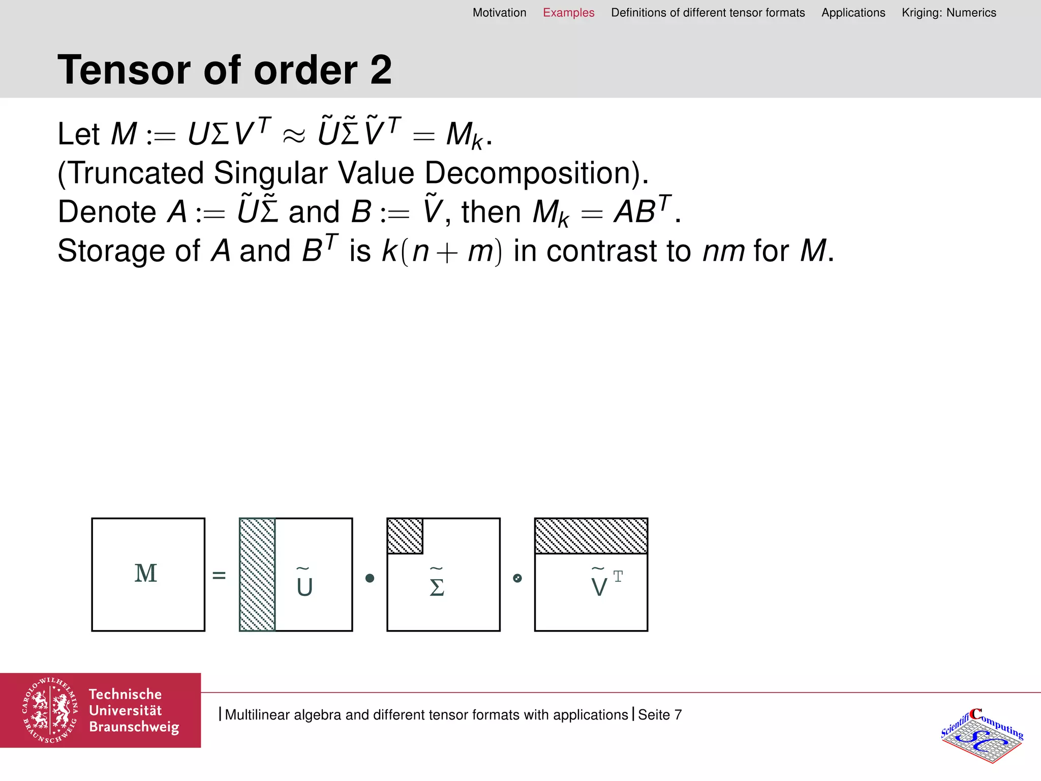
Tensor of order 2
Let M := UΣVT ≈ ˜U˜Σ˜VT = Mk.
(Truncated Singular Value Decomposition).
Denote A := ˜U˜Σ and B := ˜V, then Mk = ABT .
Storage of A and BT is k(n + m) in contrast to nm for M.
U VΣ
∼ ∼ ∼ T=M
CC
SCScientifi omputing
Multilinear algebra and different tensor formats with applications Seite 7
Motivation Examples Definitions of different tensor formats Applications Kriging: Numerics
Example: Arithmetic operations
Let v ∈ Rn.
Suppose Mk = ABT ∈ Rn×Z , A ∈ Rn×k, B ∈ RZ×k is given.
Property 1: Mkv = ABT v = (A(BT v)). Cost O(kZ + kn).
Suppose M = CDT , C ∈ Rn×k and D ∈ RZ×k.
Property 2: Mk + M = AnewBT
new, Anew := [A C] ∈ Rn×2k and
Bnew = [B D] ∈ RZ×2k.
Cost O((n + Z)k2 + k3).
CC
SCScientifi omputing
Multilinear algebra and different tensor formats with applications Seite 8
Motivation Examples Definitions of different tensor formats Applications Kriging: Numerics
Aims
1. Represent/approximate multidimensional operators and
functions in data sparse format
2. Perform linear algebra algorithms in tensor format
3. Truncate tensors to data-sparse format
4. Extract information from data-sparse solution
CC
SCScientifi omputing
Multilinear algebra and different tensor formats with applications Seite 9
Motivation Examples Definitions of different tensor formats Applications Kriging: Numerics
Definition of tensor of order d
Tensor of order d is a multidimensional array over a d-tuple index
set I = I1 × · · · × Id ,
A = [ai1...id
: i ∈ I ] ∈ RI
, I = {1, ..., n }, = 1, .., d.
A tensor A is an element of the linear space
Vn =
d
=1
V , V = RI
equipped with the Euclidean scalar product ·, · : Vn × Vn → R,
defined as
A, B :=
(i1...id )∈I
ai1...id
bi1...id
, for A, B ∈ Vn.
CC
SCScientifi omputing
Multilinear algebra and different tensor formats with applications Seite 10
Motivation Examples Definitions of different tensor formats Applications Kriging: Numerics
Rank-k representation
Tensor product of vectors u( ) = {u
( )
i }n
i =1 ∈ RI forms the
canonical rank-1 tensor
A(1) ≡ [ui]i∈I = u(1)
⊗ ... ⊗ u(d)
,
with entries ui = u
(1)
i1
⊗ ... ⊗ u
(d)
id
. The storage is dn in contrast to nd .
CC
SCScientifi omputing
Multilinear algebra and different tensor formats with applications Seite 11
Motivation Examples Definitions of different tensor formats Applications Kriging: Numerics
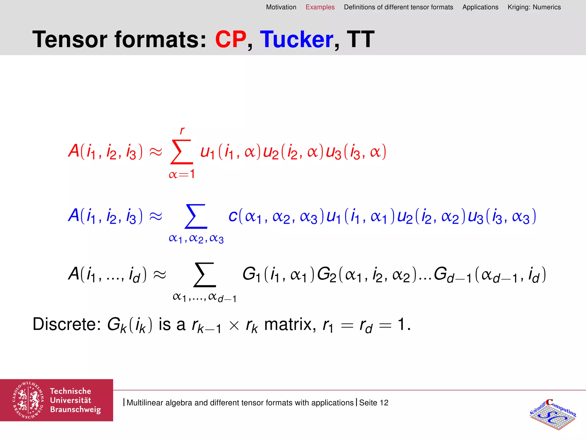
Tensor formats: CP, Tucker, TT
A(i1, i2, i3) ≈
r
α=1
u1(i1, α)u2(i2, α)u3(i3, α)
A(i1, i2, i3) ≈
α1,α2,α3
c(α1, α2, α3)u1(i1, α1)u2(i2, α2)u3(i3, α3)
A(i1, ..., id ) ≈
α1,...,αd−1
G1(i1, α1)G2(α1, i2, α2)...Gd−1(αd−1, id )
Discrete: Gk(ik) is a rk−1 × rk matrix, r1 = rd = 1.
CC
SCScientifi omputing
Multilinear algebra and different tensor formats with applications Seite 12
Motivation Examples Definitions of different tensor formats Applications Kriging: Numerics
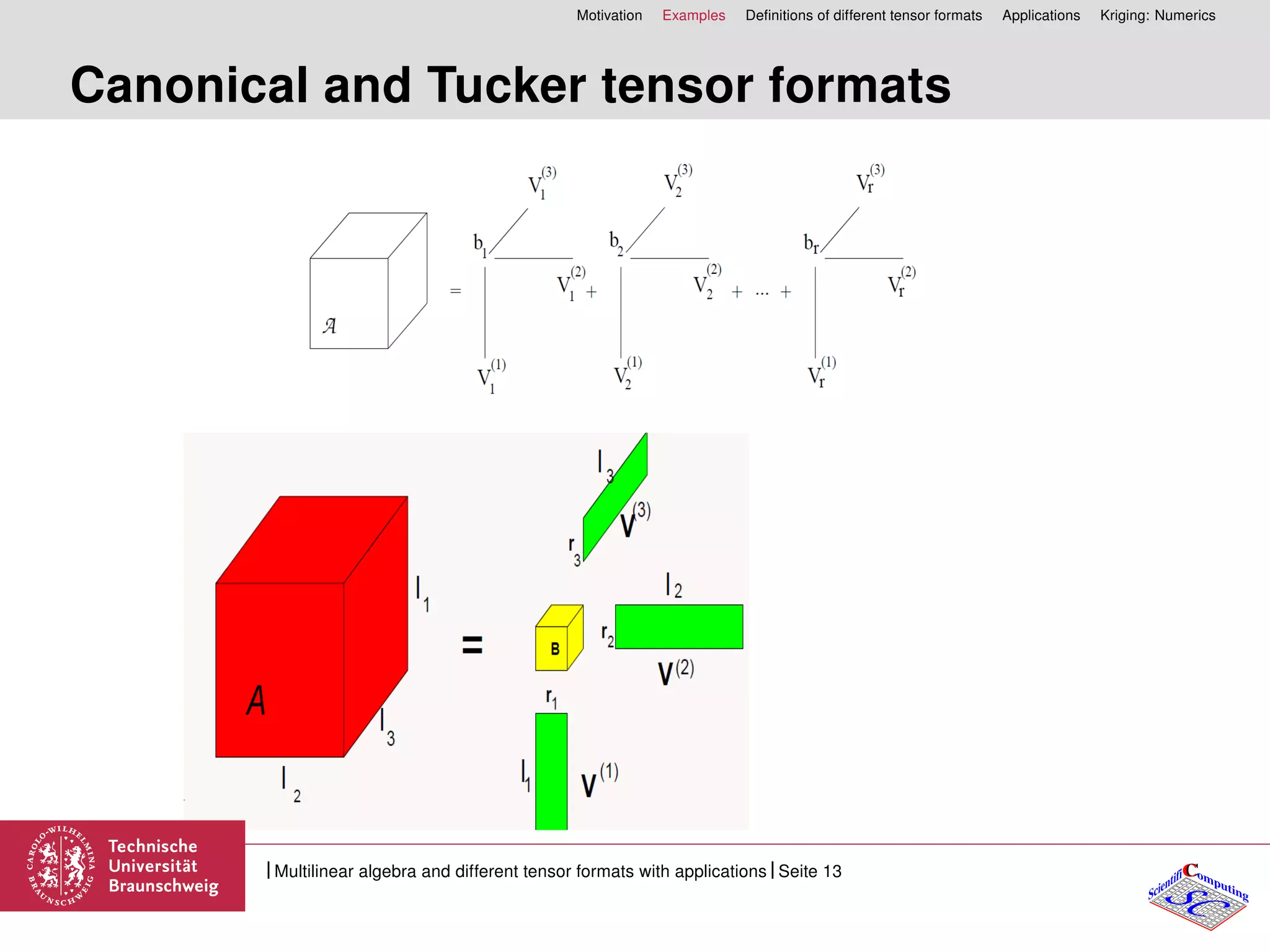
Canonical and Tucker tensor formats
CC
SCScientifi omputing
Multilinear algebra and different tensor formats with applications Seite 13
Motivation Examples Definitions of different tensor formats Applications Kriging: Numerics
Tensor and Matrices
Tensor (A ) ∈I ∈ RI
where I = I1 × I2 × ... × Id , #Iµ = nµ, #I = d
µ=1 nµ.
Rank-1 tensor
A = u1 ⊗ u2 ⊗ ... ⊗ ud =:
d
µ=1
uµ
Ai1,...,id
= (u1)i1
· ... · (ud )id
Rank-1 tensor A = u ⊗ v, matrix A = uvT , A = vuT , u ∈ Rn, v ∈ Rm,
Rank-k tensor A = k
i=1 ui ⊗ vi, matrix A = k
i=1 uivT
i .
Kronecker product A ⊗ B ∈ Rnm×nm is a block matrix whose ij-th
block is [AijB].
CC
SCScientifi omputing
Multilinear algebra and different tensor formats with applications Seite 14
Motivation Examples Definitions of different tensor formats Applications Kriging: Numerics
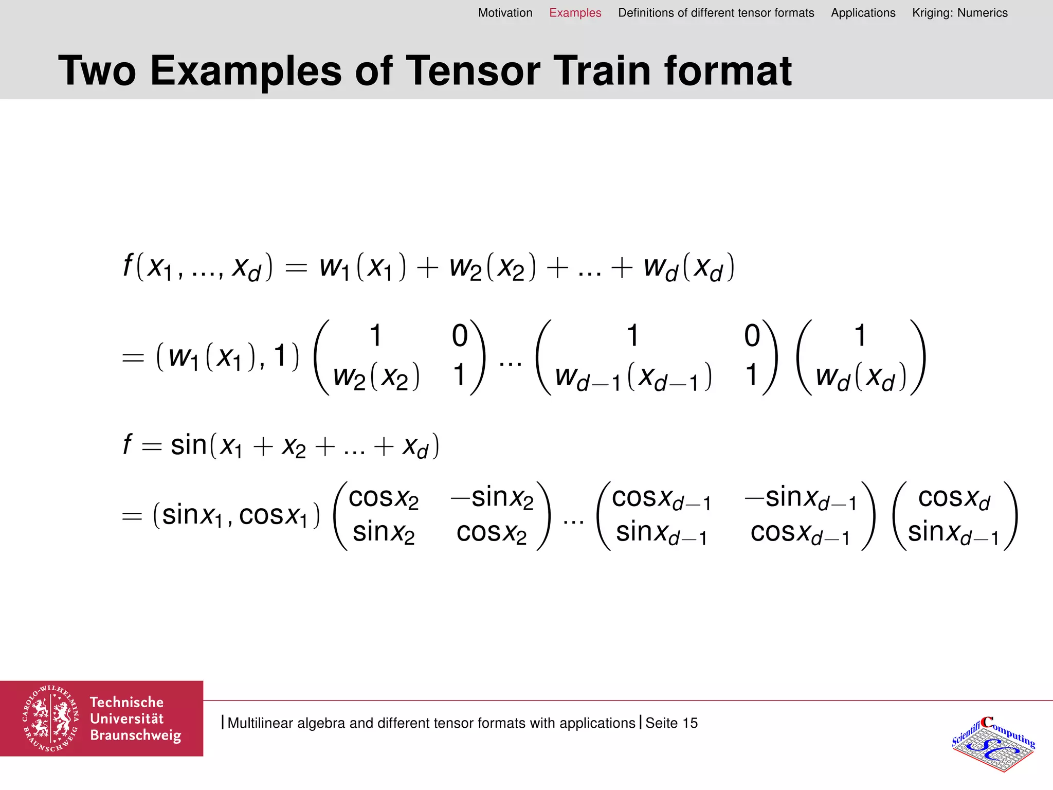
Two Examples of Tensor Train format
f(x1, ..., xd ) = w1(x1) + w2(x2) + ... + wd (xd )
= (w1(x1), 1)
1 0
w2(x2) 1
...
1 0
wd−1(xd−1) 1
1
wd (xd )
f = sin(x1 + x2 + ... + xd )
= (sinx1, cosx1)
cosx2 −sinx2
sinx2 cosx2
...
cosxd−1 −sinxd−1
sinxd−1 cosxd−1
cosxd
sinxd−1
CC
SCScientifi omputing
Multilinear algebra and different tensor formats with applications Seite 15
Motivation Examples Definitions of different tensor formats Applications Kriging: Numerics
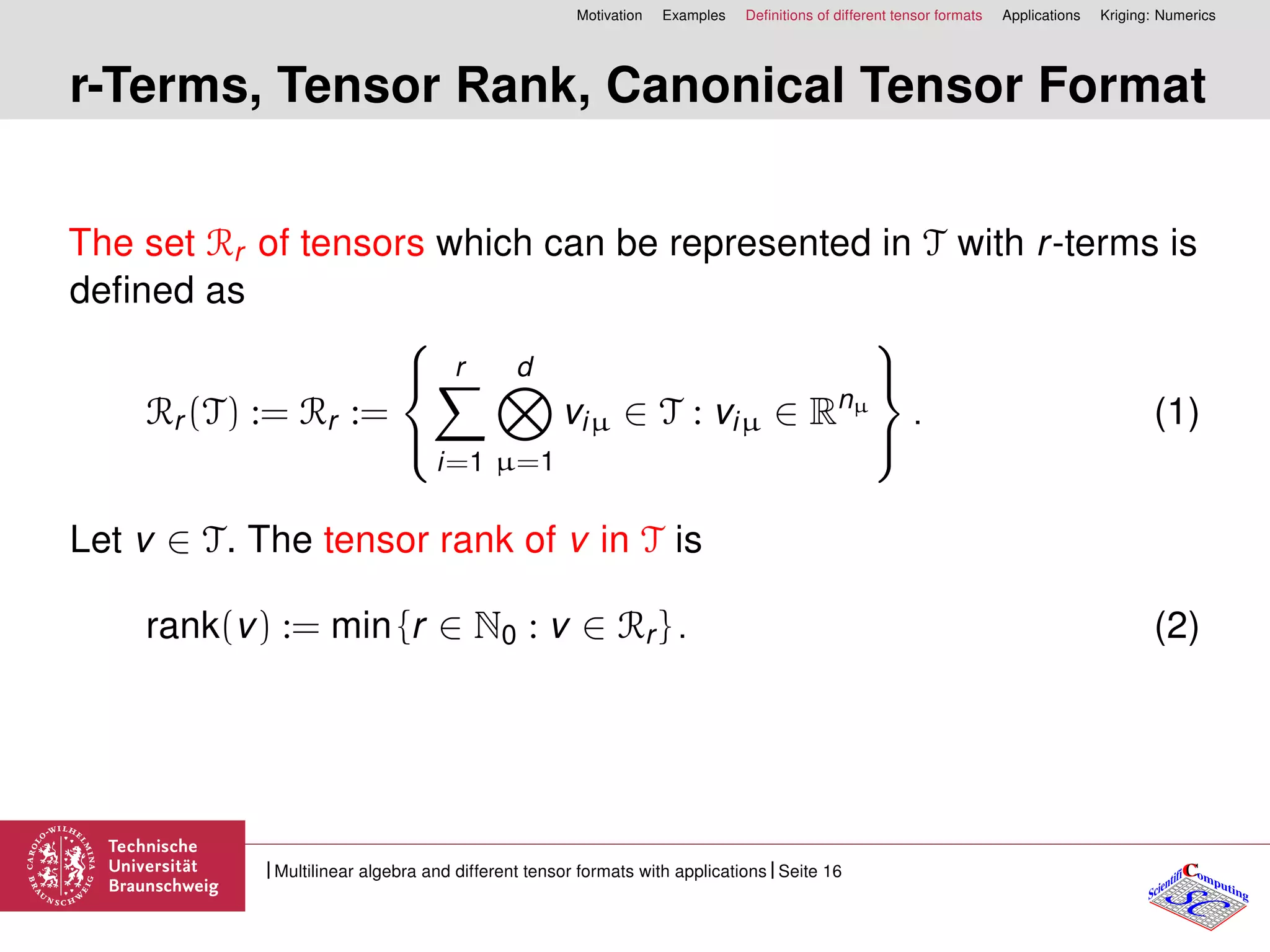
r-Terms, Tensor Rank, Canonical Tensor Format
The set Rr of tensors which can be represented in T with r-terms is
defined as
Rr (T) := Rr :=



r
i=1
d
µ=1
viµ ∈ T : viµ ∈ Rnµ



. (1)
Let v ∈ T. The tensor rank of v in T is
rank(v) := min {r ∈ N0 : v ∈ Rr } . (2)
CC
SCScientifi omputing
Multilinear algebra and different tensor formats with applications Seite 16
Motivation Examples Definitions of different tensor formats Applications Kriging: Numerics
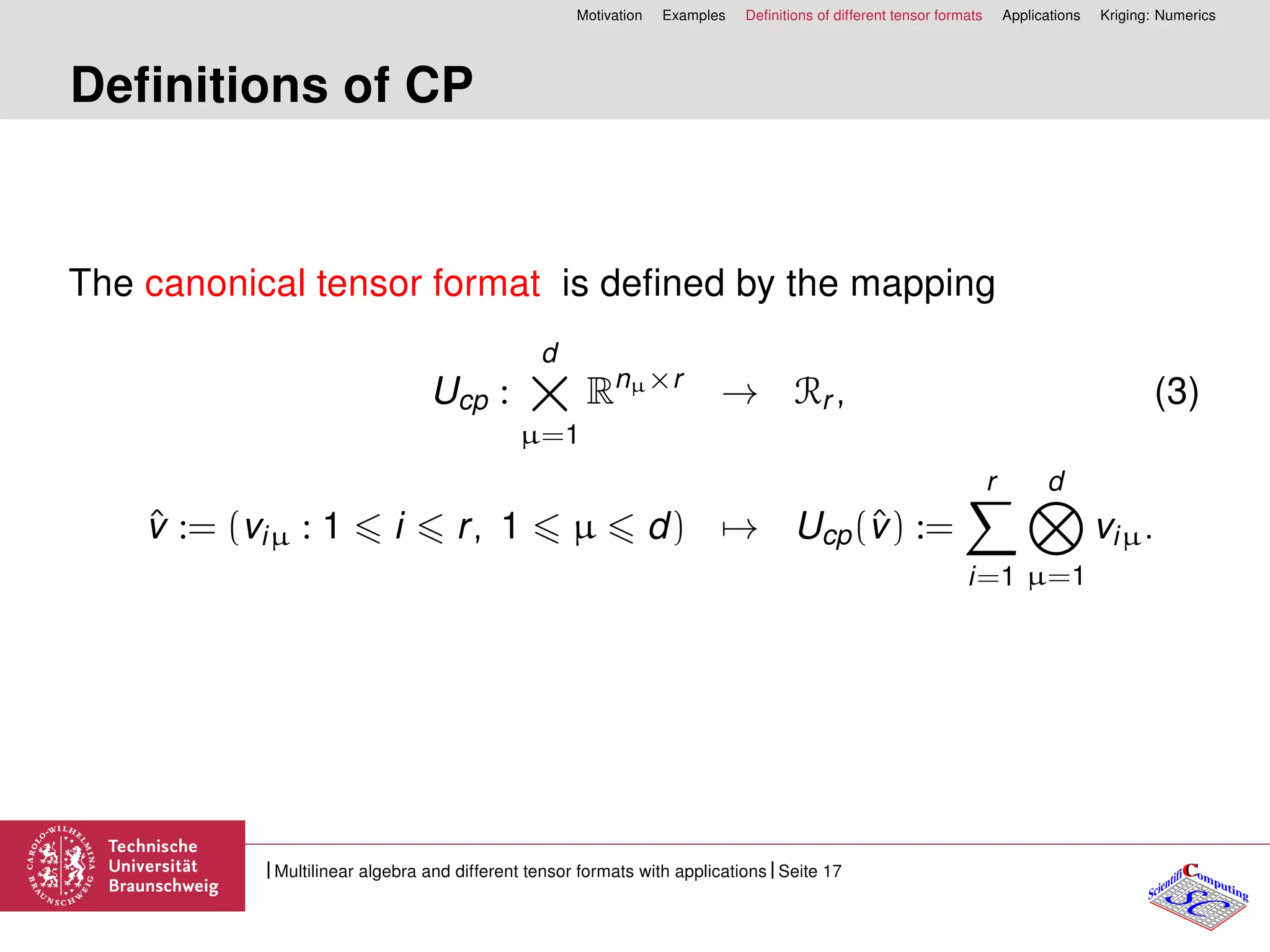
Definitions of CP
The canonical tensor format is defined by the mapping
Ucp :
d
×µ=1
Rnµ×r
→ Rr , (3)
ˆv := (viµ : 1 i r, 1 µ d) → Ucp(ˆv) :=
r
i=1
d
µ=1
viµ.
CC
SCScientifi omputing
Multilinear algebra and different tensor formats with applications Seite 17
Motivation Examples Definitions of different tensor formats Applications Kriging: Numerics
Properties of CP
Lemma
Let r1, r2 ∈ N, u ∈ Rr1
and v ∈ Rr2
. We have
(i) u, v T = r1
j1=1
r2
j2=1
d
µ=1 uj1µ, vj2µ Rnµ . The computational
cost of u, v T is O r1r2
d
µ=1 nµ .
(ii) u + v ∈ Rr1+r2
.
(iii) u v ∈ Rr1r2
, where denotes the point wise Hadamard
product. Further, u v can be computed in the canonical tensor
format with r1r2
d
µ=1 nµ arithmetic operations.
Let R1 = A1BT
1 , R2 = A2BT
2 be rank-k matrices, then
R1 + R2 = [A1A2][B1B2]T be rank-2k matrix. Rank truncation!
CC
SCScientifi omputing
Multilinear algebra and different tensor formats with applications Seite 18
Motivation Examples Definitions of different tensor formats Applications Kriging: Numerics
Properties of CP, Hadamard product and FT
Let u = k
j=1
d
i=1 uji, uji ∈ Rn.
F[d]
(˜u) =
k
j=1
d
i=1
Fi ˜uji , where F[d]
=
d
i=1
Fi. (4)
Let S = ABT = k1
i=0 aibT
i ∈ Rn×m, T = CDT = k2
j=0 cidT
i ∈ Rn×m
where ai, ci ∈ Rn, bi, di ∈ Rm, k1, k2, n, m > 0. Then
F(2)
(S ◦ T) =
k1
i=0
k2
j=0
F(ai ◦ cj)F(bT
i ◦ dT
j ).
CC
SCScientifi omputing
Multilinear algebra and different tensor formats with applications Seite 19
Motivation Examples Definitions of different tensor formats Applications Kriging: Numerics
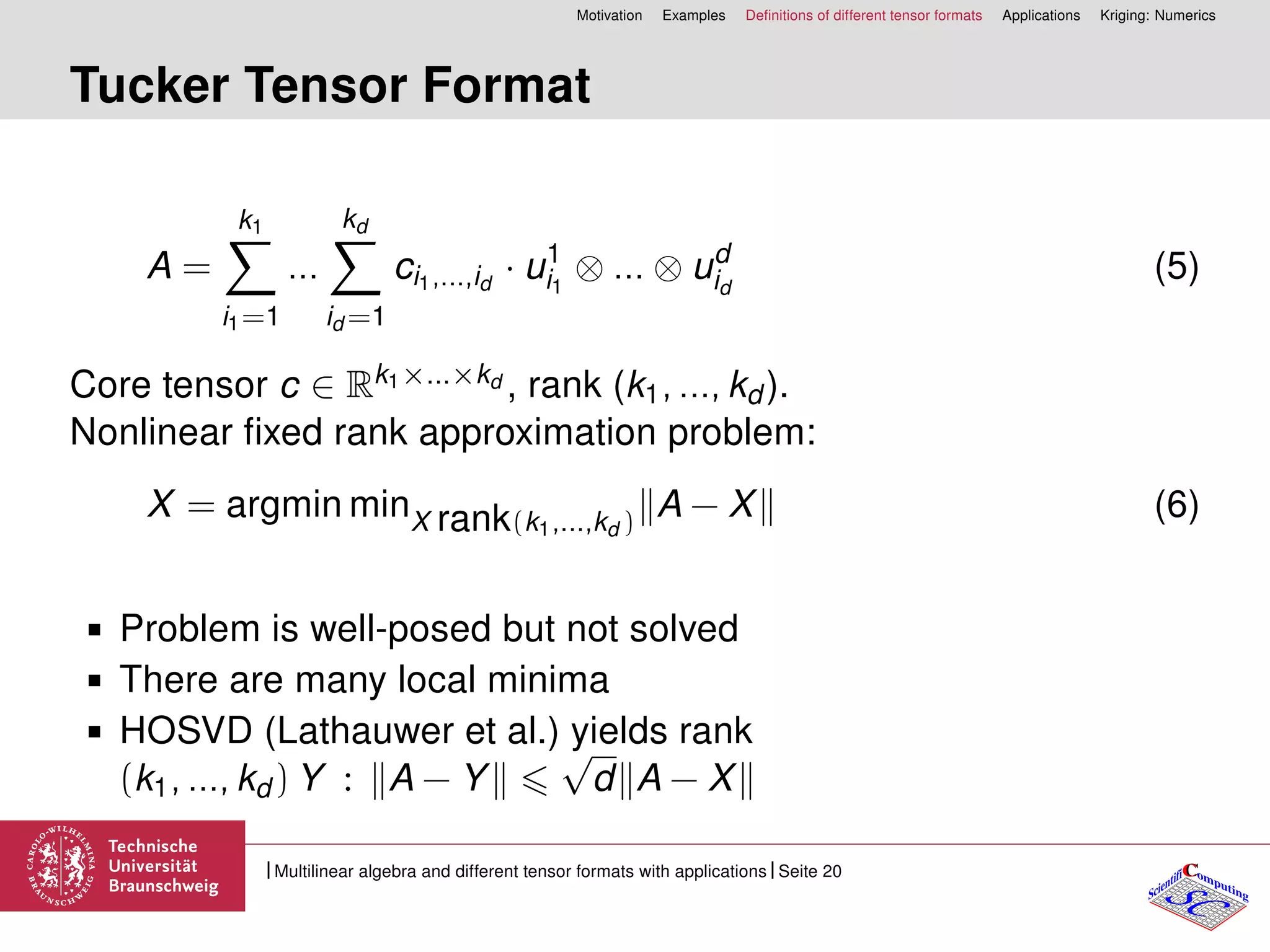
Tucker Tensor Format
A =
k1
i1=1
...
kd
id =1
ci1,...,id
· u1
i1
⊗ ... ⊗ ud
id
(5)
Core tensor c ∈ Rk1×...×kd , rank (k1, ..., kd ).
Nonlinear fixed rank approximation problem:
X = argmin minX rank(k1,...,kd )
A − X (6)
Problem is well-posed but not solved
There are many local minima
HOSVD (Lathauwer et al.) yields rank
(k1, ..., kd ) Y : A − Y
√
d A − X
CC
SCScientifi omputing
Multilinear algebra and different tensor formats with applications Seite 20
Motivation Examples Definitions of different tensor formats Applications Kriging: Numerics
Advantages and disadvantages
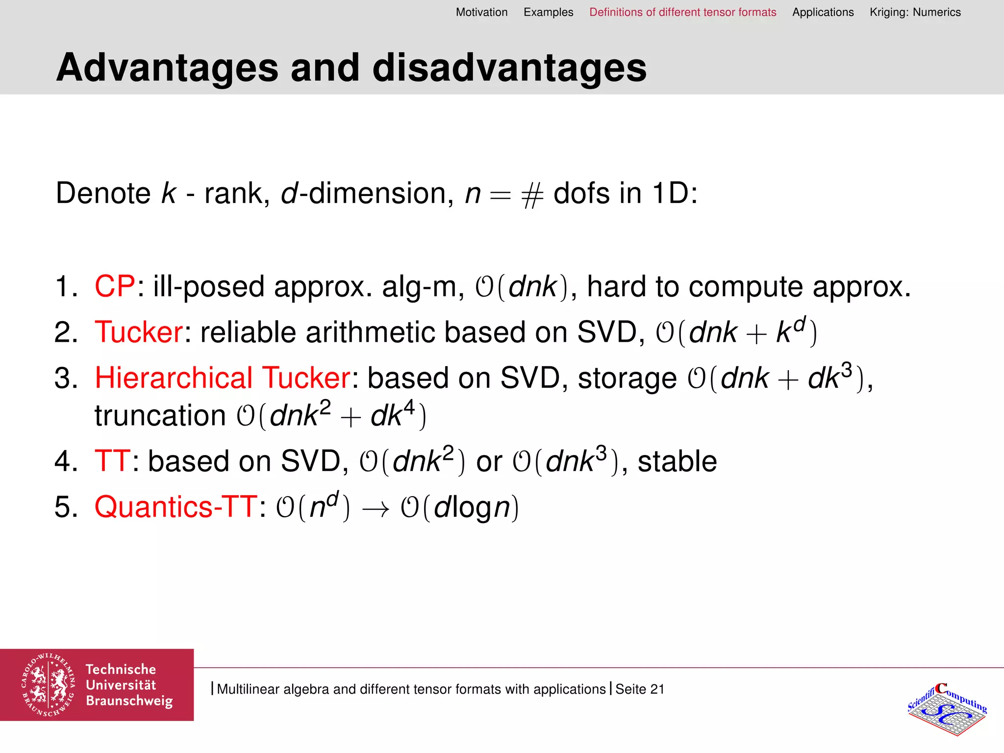
Denote k - rank, d-dimension, n = # dofs in 1D:
1. CP: ill-posed approx. alg-m, O(dnk), hard to compute approx.
2. Tucker: reliable arithmetic based on SVD, O(dnk + kd )
3. Hierarchical Tucker: based on SVD, storage O(dnk + dk3),
truncation O(dnk2 + dk4)
4. TT: based on SVD, O(dnk2) or O(dnk3), stable
5. Quantics-TT: O(nd ) → O(dlogn)
CC
SCScientifi omputing
Multilinear algebra and different tensor formats with applications Seite 21
Motivation Examples Definitions of different tensor formats Applications Kriging: Numerics
Numerics
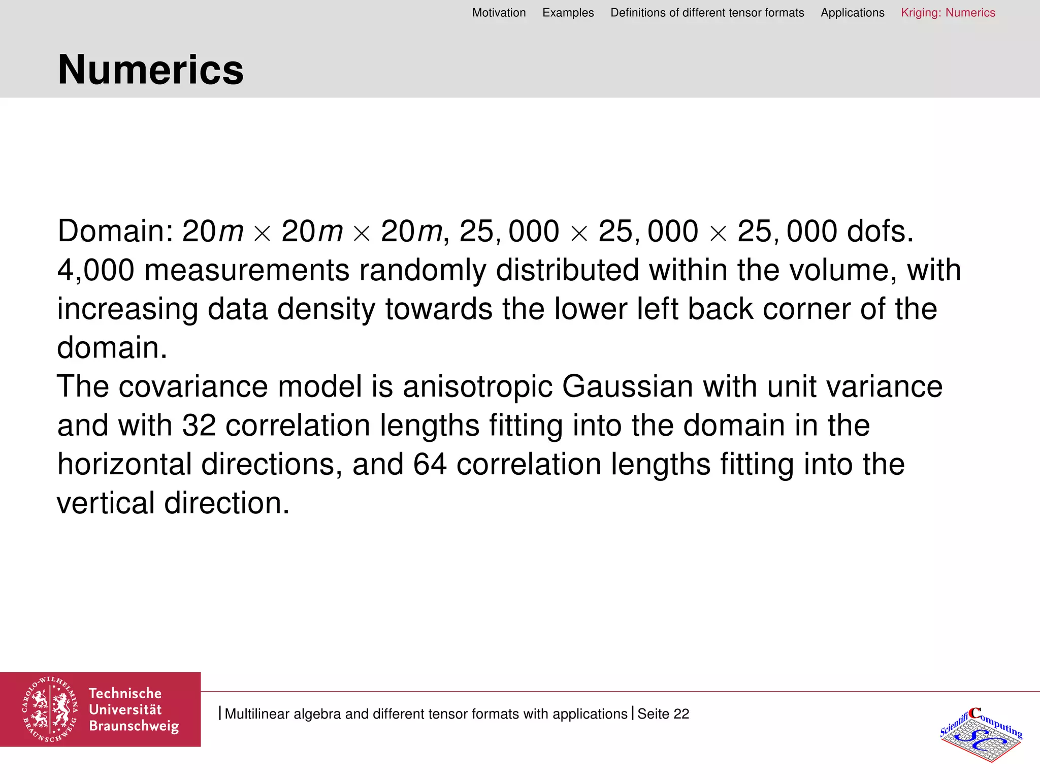
Domain: 20m × 20m × 20m, 25, 000 × 25, 000 × 25, 000 dofs.
4,000 measurements randomly distributed within the volume, with
increasing data density towards the lower left back corner of the
domain.
The covariance model is anisotropic Gaussian with unit variance
and with 32 correlation lengths fitting into the domain in the
horizontal directions, and 64 correlation lengths fitting into the
vertical direction.
CC
SCScientifi omputing
Multilinear algebra and different tensor formats with applications Seite 22
Motivation Examples Definitions of different tensor formats Applications Kriging: Numerics
Kriging: Numerics
The top left figure shows the entire domain at a sampling rate of 1:64 per
direction, and then a series of zooms into the respective lower left back
corner with zoom factors (sampling rates) of 4 (1:16), 16 (1:4), 64 (1:1) for
the top right, bottom left and bottom right plots, respectively. Color scale:
showing the 95% confidence interval [µ − 2σ, µ + 2σ].
CC
SCScientifi omputing
Multilinear algebra and different tensor formats with applications Seite 23
Motivation Examples Definitions of different tensor formats Applications Kriging: Numerics
Numerics on computer with 16GB RAM:
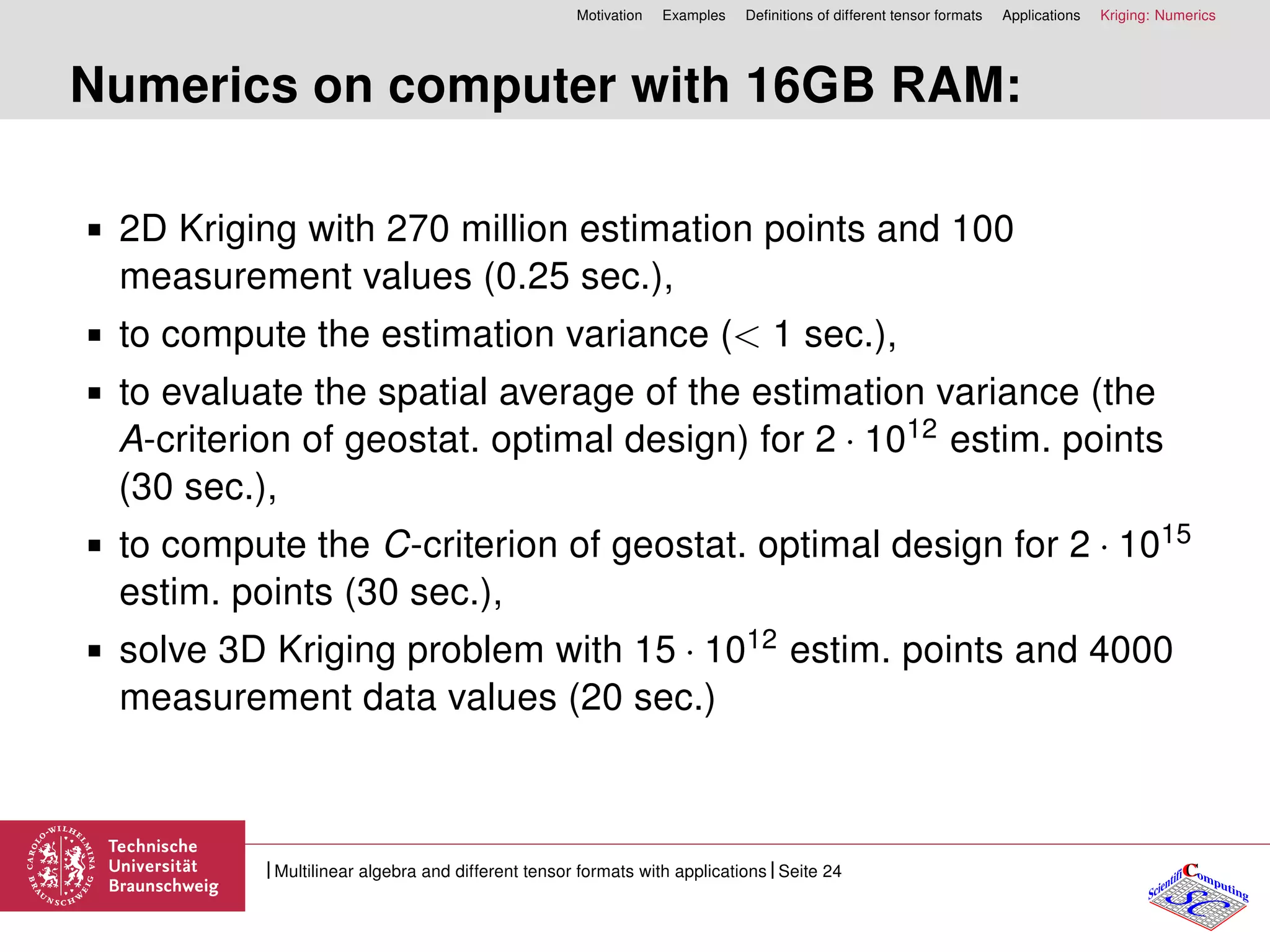
2D Kriging with 270 million estimation points and 100
measurement values (0.25 sec.),
to compute the estimation variance (< 1 sec.),
to evaluate the spatial average of the estimation variance (the
A-criterion of geostat. optimal design) for 2 · 1012 estim. points
(30 sec.),
to compute the C-criterion of geostat. optimal design for 2 · 1015
estim. points (30 sec.),
solve 3D Kriging problem with 15 · 1012 estim. points and 4000
measurement data values (20 sec.)
CC
SCScientifi omputing
Multilinear algebra and different tensor formats with applications Seite 24
Motivation Examples Definitions of different tensor formats Applications Kriging: Numerics
Conclusion
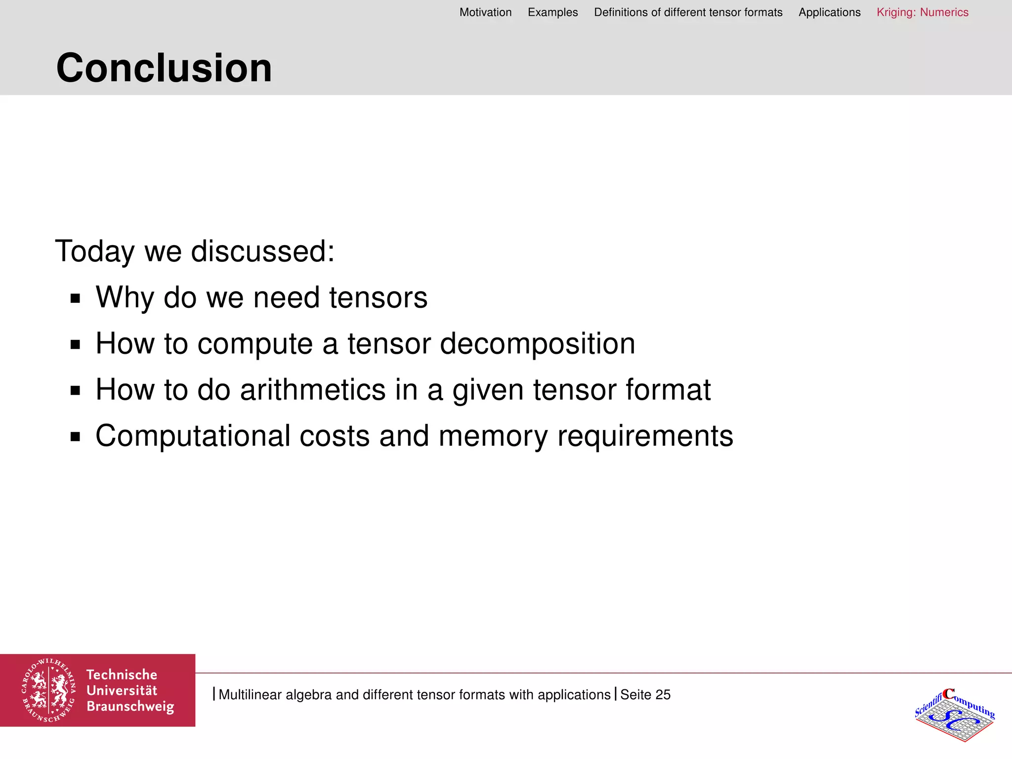
Today we discussed:
Why do we need tensors
How to compute a tensor decomposition
How to do arithmetics in a given tensor format
Computational costs and memory requirements
CC
SCScientifi omputing
Multilinear algebra and different tensor formats with applications Seite 25
Motivation Examples Definitions of different tensor formats Applications Kriging: Numerics
Tensor Software
D.Kressner, C. Tobler, Hierarchical Tucker Toolbox (Matlab),
http://www.sam.math.ethz.ch/NLAgroup/htucker_toolbox.html
M. Espig, et al
Tensor Calculus library (C): http://gitorious.org/tensorcalculus
CC
SCScientifi omputing
Multilinear algebra and different tensor formats with applications Seite 26

Multi-linear algebra and different tensor formats with applications

  • 1.
    Multilinear algebra anddifferent tensor formats with applications A. Litvinenko, litvinen@tu-bs.de, 12. Juni 2013 CC SCScientifi omputing
  • 2.
    Motivation Examples Definitionsof different tensor formats Applications Kriging: Numerics Outline Motivation Numerical Experiments Examples Definitions of different tensor formats Applications Kriging: Numerics CC SCScientifi omputing Multilinear algebra and different tensor formats with applications Seite 2
  • 3.
    Motivation Examples Definitionsof different tensor formats Applications Kriging: Numerics Used Literature and Slides Book of W. Hackbusch 2012, Dissertations of I. Oseledets and M. Espig Articles of Tyrtyshnikov et al., De Lathauwer et al., L. Grasedyck, B. Khoromskij, M. Espig Lecture courses and presentations of Boris and Venera Khoromskij Software T. Kolda, M. Espig et al.; D. Kressner, K. Tobler; I. Oseledets et al. CC SCScientifi omputing Multilinear algebra and different tensor formats with applications Seite 3
  • 4.
    Motivation Examples Definitionsof different tensor formats Applications Kriging: Numerics Numerical Experiments Challenges of numerical computations modelling of multi-particle interactions in large molecular systems such as proteins, biomolecules, modelling of large atomic (metallic) clusters, stochastic and parametric equations, machine learning, data mining and information technologies, multidimensional dynamical systems, data compression financial mathematics, analysis of multi-dimensional data. CC SCScientifi omputing Multilinear algebra and different tensor formats with applications Seite 4
  • 5.
    Motivation Examples Definitionsof different tensor formats Applications Kriging: Numerics Numerical Experiments Example: Final discretized stochastic PDE Au = f, where A:= s l=1 ˜Al ⊗ M µ=1 ∆lµ , ˜Al ∈ RN×N, ∆lµ ∈ RRµ×Rµ , u:= r j=1 uj ⊗ M µ=1 ujµ , uj ∈ RN, ujµ ∈ RRµ , f:= R k=1 ˜fk ⊗ M µ=1 gkµ, ˜fk ∈ RN and gkµ ∈ RRµ . And then solve iteratively with a tensor preconditioner [PhD of E. Zander, 2012] [Wähnert, Espig, Hackbusch, Litvinenko, Matthies 05.2012] CC SCScientifi omputing Multilinear algebra and different tensor formats with applications Seite 5
  • 6.
    Motivation Examples Definitionsof different tensor formats Applications Kriging: Numerics Numerical Experiments Numerical example 2D L-shape domain, N = 557. Total stoch. dim. Mu = Mk + Mf = 20, |J| = 231 Solve linear system above, obtain solution in a tensor format: u = 231 j=1 21 µ=1 ujµ ∈ R557 ⊗ 20 µ=1 R3. Tensor u has 320 ∗ 557 ≈ 2 · 1012 entries. Memory cost 16 TB. Want to compute maximum element of u Want to compute all elements of u from e.g. the interval [0.2, 0.4] (did in 10 minutes). CC SCScientifi omputing Multilinear algebra and different tensor formats with applications Seite 6
  • 7.
    Motivation Examples Definitionsof different tensor formats Applications Kriging: Numerics Tensor of order 2 Let M := UΣVT ≈ ˜U˜Σ˜VT = Mk. (Truncated Singular Value Decomposition). Denote A := ˜U˜Σ and B := ˜V, then Mk = ABT . Storage of A and BT is k(n + m) in contrast to nm for M. U VΣ ∼ ∼ ∼ T=M CC SCScientifi omputing Multilinear algebra and different tensor formats with applications Seite 7
  • 8.
    Motivation Examples Definitionsof different tensor formats Applications Kriging: Numerics Example: Arithmetic operations Let v ∈ Rn. Suppose Mk = ABT ∈ Rn×Z , A ∈ Rn×k, B ∈ RZ×k is given. Property 1: Mkv = ABT v = (A(BT v)). Cost O(kZ + kn). Suppose M = CDT , C ∈ Rn×k and D ∈ RZ×k. Property 2: Mk + M = AnewBT new, Anew := [A C] ∈ Rn×2k and Bnew = [B D] ∈ RZ×2k. Cost O((n + Z)k2 + k3). CC SCScientifi omputing Multilinear algebra and different tensor formats with applications Seite 8
  • 9.
    Motivation Examples Definitionsof different tensor formats Applications Kriging: Numerics Aims 1. Represent/approximate multidimensional operators and functions in data sparse format 2. Perform linear algebra algorithms in tensor format 3. Truncate tensors to data-sparse format 4. Extract information from data-sparse solution CC SCScientifi omputing Multilinear algebra and different tensor formats with applications Seite 9
  • 10.
    Motivation Examples Definitionsof different tensor formats Applications Kriging: Numerics Definition of tensor of order d Tensor of order d is a multidimensional array over a d-tuple index set I = I1 × · · · × Id , A = [ai1...id : i ∈ I ] ∈ RI , I = {1, ..., n }, = 1, .., d. A tensor A is an element of the linear space Vn = d =1 V , V = RI equipped with the Euclidean scalar product ·, · : Vn × Vn → R, defined as A, B := (i1...id )∈I ai1...id bi1...id , for A, B ∈ Vn. CC SCScientifi omputing Multilinear algebra and different tensor formats with applications Seite 10
  • 11.
    Motivation Examples Definitionsof different tensor formats Applications Kriging: Numerics Rank-k representation Tensor product of vectors u( ) = {u ( ) i }n i =1 ∈ RI forms the canonical rank-1 tensor A(1) ≡ [ui]i∈I = u(1) ⊗ ... ⊗ u(d) , with entries ui = u (1) i1 ⊗ ... ⊗ u (d) id . The storage is dn in contrast to nd . CC SCScientifi omputing Multilinear algebra and different tensor formats with applications Seite 11
  • 12.
    Motivation Examples Definitionsof different tensor formats Applications Kriging: Numerics Tensor formats: CP, Tucker, TT A(i1, i2, i3) ≈ r α=1 u1(i1, α)u2(i2, α)u3(i3, α) A(i1, i2, i3) ≈ α1,α2,α3 c(α1, α2, α3)u1(i1, α1)u2(i2, α2)u3(i3, α3) A(i1, ..., id ) ≈ α1,...,αd−1 G1(i1, α1)G2(α1, i2, α2)...Gd−1(αd−1, id ) Discrete: Gk(ik) is a rk−1 × rk matrix, r1 = rd = 1. CC SCScientifi omputing Multilinear algebra and different tensor formats with applications Seite 12
  • 13.
    Motivation Examples Definitionsof different tensor formats Applications Kriging: Numerics Canonical and Tucker tensor formats CC SCScientifi omputing Multilinear algebra and different tensor formats with applications Seite 13
  • 14.
    Motivation Examples Definitionsof different tensor formats Applications Kriging: Numerics Tensor and Matrices Tensor (A ) ∈I ∈ RI where I = I1 × I2 × ... × Id , #Iµ = nµ, #I = d µ=1 nµ. Rank-1 tensor A = u1 ⊗ u2 ⊗ ... ⊗ ud =: d µ=1 uµ Ai1,...,id = (u1)i1 · ... · (ud )id Rank-1 tensor A = u ⊗ v, matrix A = uvT , A = vuT , u ∈ Rn, v ∈ Rm, Rank-k tensor A = k i=1 ui ⊗ vi, matrix A = k i=1 uivT i . Kronecker product A ⊗ B ∈ Rnm×nm is a block matrix whose ij-th block is [AijB]. CC SCScientifi omputing Multilinear algebra and different tensor formats with applications Seite 14
  • 15.
    Motivation Examples Definitionsof different tensor formats Applications Kriging: Numerics Two Examples of Tensor Train format f(x1, ..., xd ) = w1(x1) + w2(x2) + ... + wd (xd ) = (w1(x1), 1) 1 0 w2(x2) 1 ... 1 0 wd−1(xd−1) 1 1 wd (xd ) f = sin(x1 + x2 + ... + xd ) = (sinx1, cosx1) cosx2 −sinx2 sinx2 cosx2 ... cosxd−1 −sinxd−1 sinxd−1 cosxd−1 cosxd sinxd−1 CC SCScientifi omputing Multilinear algebra and different tensor formats with applications Seite 15
  • 16.
    Motivation Examples Definitionsof different tensor formats Applications Kriging: Numerics r-Terms, Tensor Rank, Canonical Tensor Format The set Rr of tensors which can be represented in T with r-terms is defined as Rr (T) := Rr :=    r i=1 d µ=1 viµ ∈ T : viµ ∈ Rnµ    . (1) Let v ∈ T. The tensor rank of v in T is rank(v) := min {r ∈ N0 : v ∈ Rr } . (2) CC SCScientifi omputing Multilinear algebra and different tensor formats with applications Seite 16
  • 17.
    Motivation Examples Definitionsof different tensor formats Applications Kriging: Numerics Definitions of CP The canonical tensor format is defined by the mapping Ucp : d ×µ=1 Rnµ×r → Rr , (3) ˆv := (viµ : 1 i r, 1 µ d) → Ucp(ˆv) := r i=1 d µ=1 viµ. CC SCScientifi omputing Multilinear algebra and different tensor formats with applications Seite 17
  • 18.
    Motivation Examples Definitionsof different tensor formats Applications Kriging: Numerics Properties of CP Lemma Let r1, r2 ∈ N, u ∈ Rr1 and v ∈ Rr2 . We have (i) u, v T = r1 j1=1 r2 j2=1 d µ=1 uj1µ, vj2µ Rnµ . The computational cost of u, v T is O r1r2 d µ=1 nµ . (ii) u + v ∈ Rr1+r2 . (iii) u v ∈ Rr1r2 , where denotes the point wise Hadamard product. Further, u v can be computed in the canonical tensor format with r1r2 d µ=1 nµ arithmetic operations. Let R1 = A1BT 1 , R2 = A2BT 2 be rank-k matrices, then R1 + R2 = [A1A2][B1B2]T be rank-2k matrix. Rank truncation! CC SCScientifi omputing Multilinear algebra and different tensor formats with applications Seite 18
  • 19.
    Motivation Examples Definitionsof different tensor formats Applications Kriging: Numerics Properties of CP, Hadamard product and FT Let u = k j=1 d i=1 uji, uji ∈ Rn. F[d] (˜u) = k j=1 d i=1 Fi ˜uji , where F[d] = d i=1 Fi. (4) Let S = ABT = k1 i=0 aibT i ∈ Rn×m, T = CDT = k2 j=0 cidT i ∈ Rn×m where ai, ci ∈ Rn, bi, di ∈ Rm, k1, k2, n, m > 0. Then F(2) (S ◦ T) = k1 i=0 k2 j=0 F(ai ◦ cj)F(bT i ◦ dT j ). CC SCScientifi omputing Multilinear algebra and different tensor formats with applications Seite 19
  • 20.
    Motivation Examples Definitionsof different tensor formats Applications Kriging: Numerics Tucker Tensor Format A = k1 i1=1 ... kd id =1 ci1,...,id · u1 i1 ⊗ ... ⊗ ud id (5) Core tensor c ∈ Rk1×...×kd , rank (k1, ..., kd ). Nonlinear fixed rank approximation problem: X = argmin minX rank(k1,...,kd ) A − X (6) Problem is well-posed but not solved There are many local minima HOSVD (Lathauwer et al.) yields rank (k1, ..., kd ) Y : A − Y √ d A − X CC SCScientifi omputing Multilinear algebra and different tensor formats with applications Seite 20
  • 21.
    Motivation Examples Definitionsof different tensor formats Applications Kriging: Numerics Advantages and disadvantages Denote k - rank, d-dimension, n = # dofs in 1D: 1. CP: ill-posed approx. alg-m, O(dnk), hard to compute approx. 2. Tucker: reliable arithmetic based on SVD, O(dnk + kd ) 3. Hierarchical Tucker: based on SVD, storage O(dnk + dk3), truncation O(dnk2 + dk4) 4. TT: based on SVD, O(dnk2) or O(dnk3), stable 5. Quantics-TT: O(nd ) → O(dlogn) CC SCScientifi omputing Multilinear algebra and different tensor formats with applications Seite 21
  • 22.
    Motivation Examples Definitionsof different tensor formats Applications Kriging: Numerics Numerics Domain: 20m × 20m × 20m, 25, 000 × 25, 000 × 25, 000 dofs. 4,000 measurements randomly distributed within the volume, with increasing data density towards the lower left back corner of the domain. The covariance model is anisotropic Gaussian with unit variance and with 32 correlation lengths fitting into the domain in the horizontal directions, and 64 correlation lengths fitting into the vertical direction. CC SCScientifi omputing Multilinear algebra and different tensor formats with applications Seite 22
  • 23.
    Motivation Examples Definitionsof different tensor formats Applications Kriging: Numerics Kriging: Numerics The top left figure shows the entire domain at a sampling rate of 1:64 per direction, and then a series of zooms into the respective lower left back corner with zoom factors (sampling rates) of 4 (1:16), 16 (1:4), 64 (1:1) for the top right, bottom left and bottom right plots, respectively. Color scale: showing the 95% confidence interval [µ − 2σ, µ + 2σ]. CC SCScientifi omputing Multilinear algebra and different tensor formats with applications Seite 23
  • 24.
    Motivation Examples Definitionsof different tensor formats Applications Kriging: Numerics Numerics on computer with 16GB RAM: 2D Kriging with 270 million estimation points and 100 measurement values (0.25 sec.), to compute the estimation variance (< 1 sec.), to evaluate the spatial average of the estimation variance (the A-criterion of geostat. optimal design) for 2 · 1012 estim. points (30 sec.), to compute the C-criterion of geostat. optimal design for 2 · 1015 estim. points (30 sec.), solve 3D Kriging problem with 15 · 1012 estim. points and 4000 measurement data values (20 sec.) CC SCScientifi omputing Multilinear algebra and different tensor formats with applications Seite 24
  • 25.
    Motivation Examples Definitionsof different tensor formats Applications Kriging: Numerics Conclusion Today we discussed: Why do we need tensors How to compute a tensor decomposition How to do arithmetics in a given tensor format Computational costs and memory requirements CC SCScientifi omputing Multilinear algebra and different tensor formats with applications Seite 25
  • 26.
    Motivation Examples Definitionsof different tensor formats Applications Kriging: Numerics Tensor Software D.Kressner, C. Tobler, Hierarchical Tucker Toolbox (Matlab), http://www.sam.math.ethz.ch/NLAgroup/htucker_toolbox.html M. Espig, et al Tensor Calculus library (C): http://gitorious.org/tensorcalculus CC SCScientifi omputing Multilinear algebra and different tensor formats with applications Seite 26