This document discusses data warehousing and multi-dimensional data structures. It explains that multi-dimensional structures store data and relationships in a cube format, with each dimension side of the cube. Cubes allow for pre-aggregation of data to speed up complex queries. Common analytical operations on cubes include consolidation, drill-down, slicing, dicing, and pivoting of the data in the cube. Pre-aggregation and sparse data storage techniques reduce the overall cube size and processing needs.

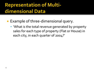
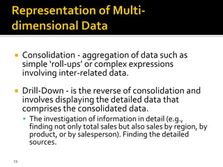
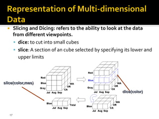
1. DATA WAREHOUSING
Multi Dimensional
OLAP

2. Usando el
DW
2

3. 3

4.  Example of two-dimensional query.
▪ What is the total revenue generated by property sales in
each city, in each quarter of 2004?’
 Choice of representation is based on types of
queries end-user may ask.
4

5. Compare representation - three-field relational table versus two-
dimensional matrix.
5

6.  Example of three-dimensional query.
 ‘What is the total revenue generated by property
sales for each type of property (Flat or House) in
each city, in each quarter of 2004?’
6

7. Data Cube
Compare representation - four-field relational table versus three-dimensional cube.
7

8.  A subset of highly interrelated data that is
organized to allow users to combine any
attributes in a cube (e.g., stores, products,
customers, suppliers) with any metrics in the
cube (e.g., sales, profit, units, age) to create
various two-dimensional views, or slices, that
can be displayed on a computer screen
8

9.  Cube represents data as cells in an array.
 Relational table only represents multi-
dimensional data in two dimensions.
9

10.  Use multi-dimensional structures to store
data and relationships between data.
 Multi-dimensional structures are best
visualized as cubes of data, and cubes within
cubes of data. Each side of a cube is a
dimension.
 A cube can be expanded to include other
dimensions.
10

11.  A cube supports matrix arithmetic.
 Multi-dimensional query response time
depends on how many cells have to be added
‘on the fly’.
 As number of dimensions increases, number
of the cube’s cells increases exponentially.
11

12.  However, majority of multi-dimensional
queries use summarized, high-level data.
 Solution is to pre-aggregate (consolidate) all
logical subtotals and totals along all
dimensions.
12

13.  Pre-aggregation is valuable, as typical
dimensions are hierarchical in nature.
 (e.g. Time dimension hierarchy - years, quarters,
months, weeks, and days)
 Predefined hierarchy allows logical pre-
aggregation and, conversely, allows for a
logical ‘drill-down’.
13

14.  Supports common analytical operations
 Consolidation
 Drill-down
 Slicing and dicing
 Pivoting
14

15.  Consolidation - aggregation of data such as
simple ‘roll-ups’ or complex expressions
involving inter-related data.
 Drill-Down - is the reverse of consolidation and
involves displaying the detailed data that
comprises the consolidated data.
 The investigation of information in detail (e.g.,
finding not only total sales but also sales by region, by
product, or by salesperson). Finding the detailed
sources.
15

16. 16

17.  Slicing and Dicing: refers to the ability to look at the data
from different viewpoints.
 dice: to cut into small cubes
 slice: A section of an cube selected by specifying its lower and
upper limits
slice(color,mes)
dice(color)
17

18.  Pivoting:
 Pivot deals with presentation
 Choose some dimensions X1, . . . ,Xi to appear
on x and some dims Y1, . . . ,Yj to appear on y.
18

19.  Can store data in a compressed form by dynamically
selecting physical storage organizations and compression
techniques that maximize space utilization.
 Dense data (that is, data that exists for a high percentage of
cells) can be stored separately from sparse data (that is, a
significant percentage of cells are empty).
19

20.  Ability to omit empty or repetitive cells can
greatly reduce the size of the cube and the
amount of processing.
 Allows analysis of exceptionally large
amounts of data.
20

21.  In summary, pre-aggregation, dimensional
hierarchy, and sparse data management can
significantly reduce the size of the cube and
the need to calculate values ‘on-the-fly’.
 Removes need for multi-table joins and
provides quick and direct access to arrays of
data, thus significantly speeding up
execution of multi-dimensional queries.
21

22.  Efraim Turban. Business Intelligence. Prentice
Hall.2008.