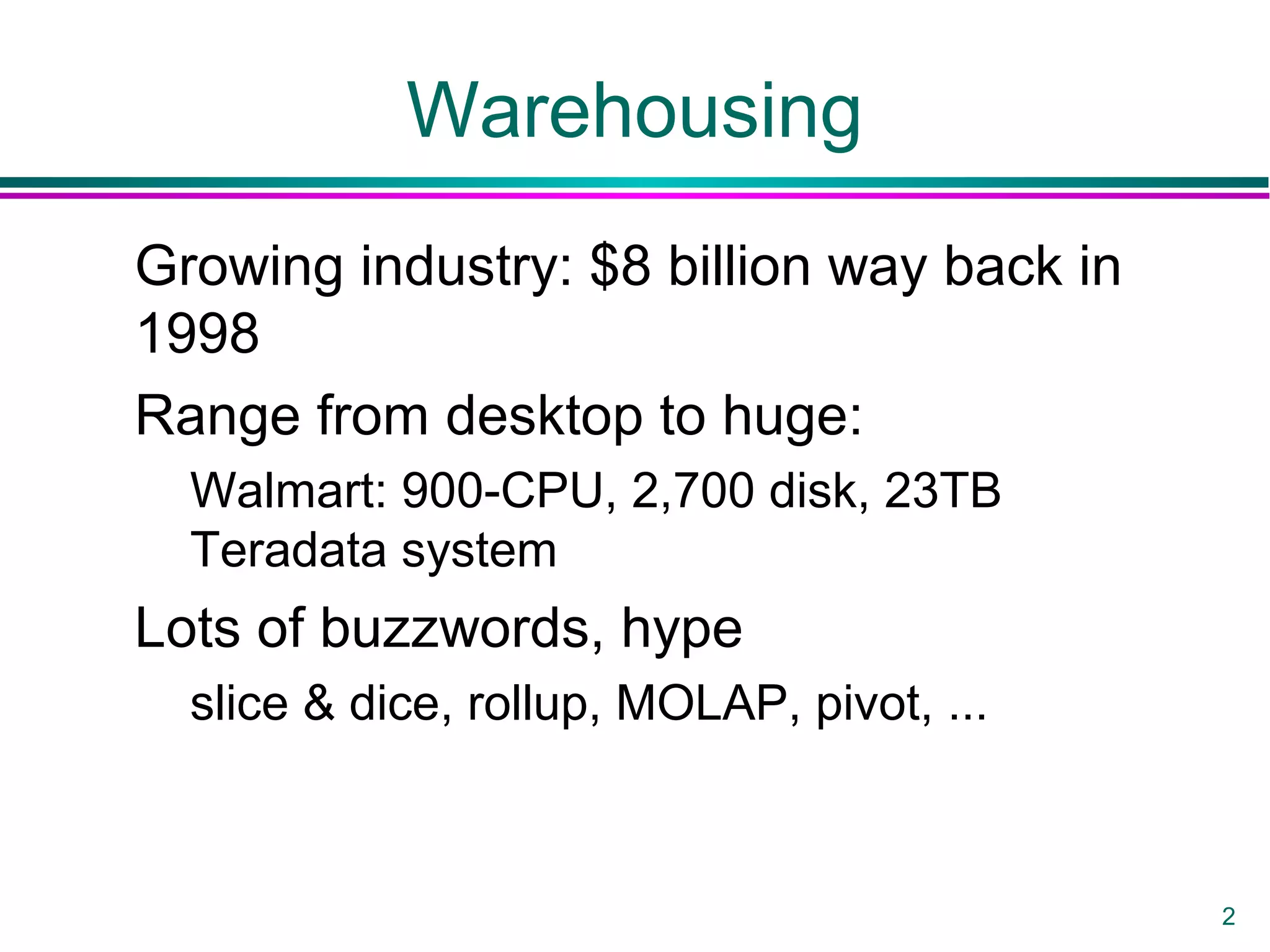
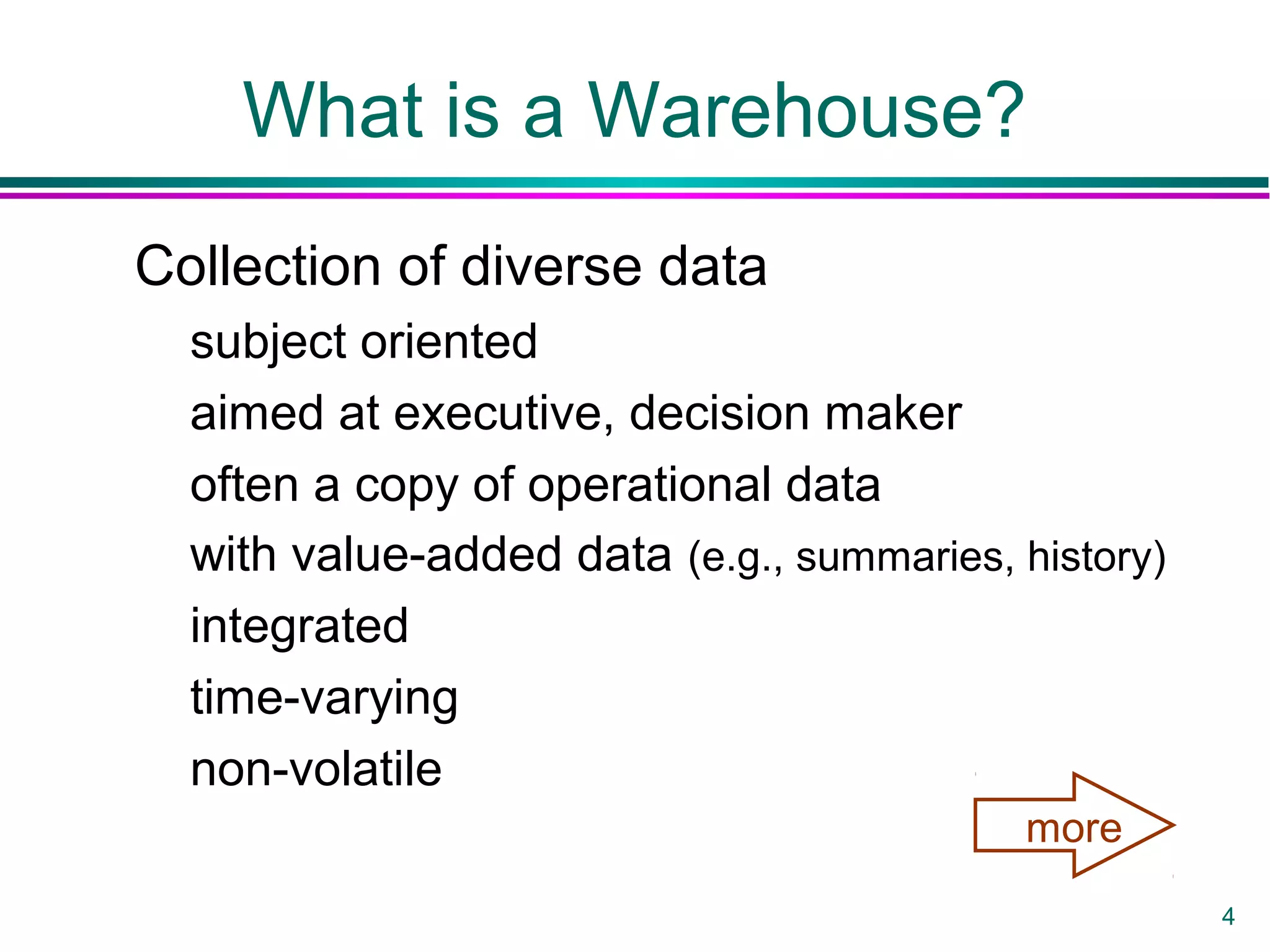
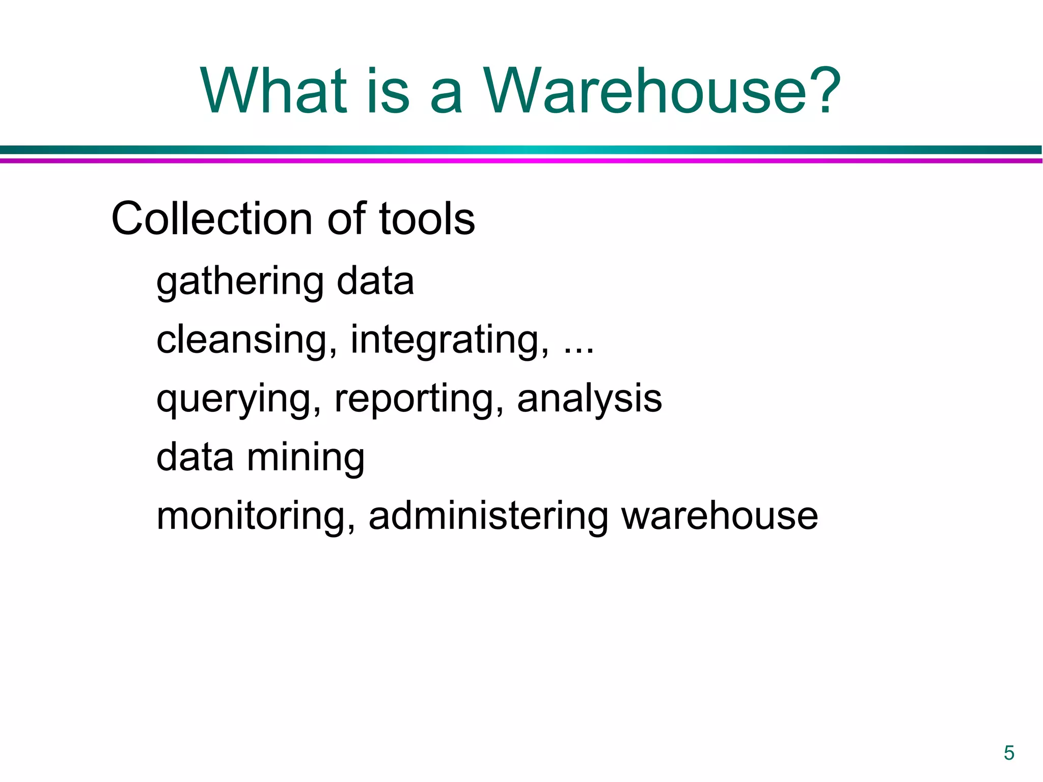
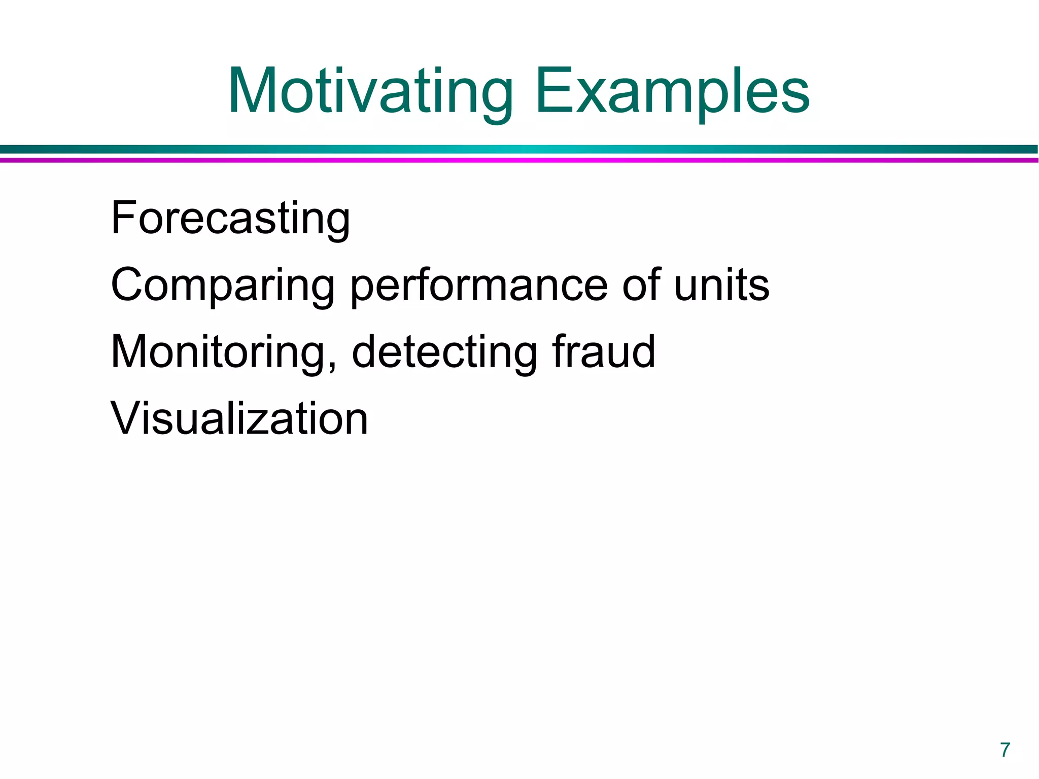
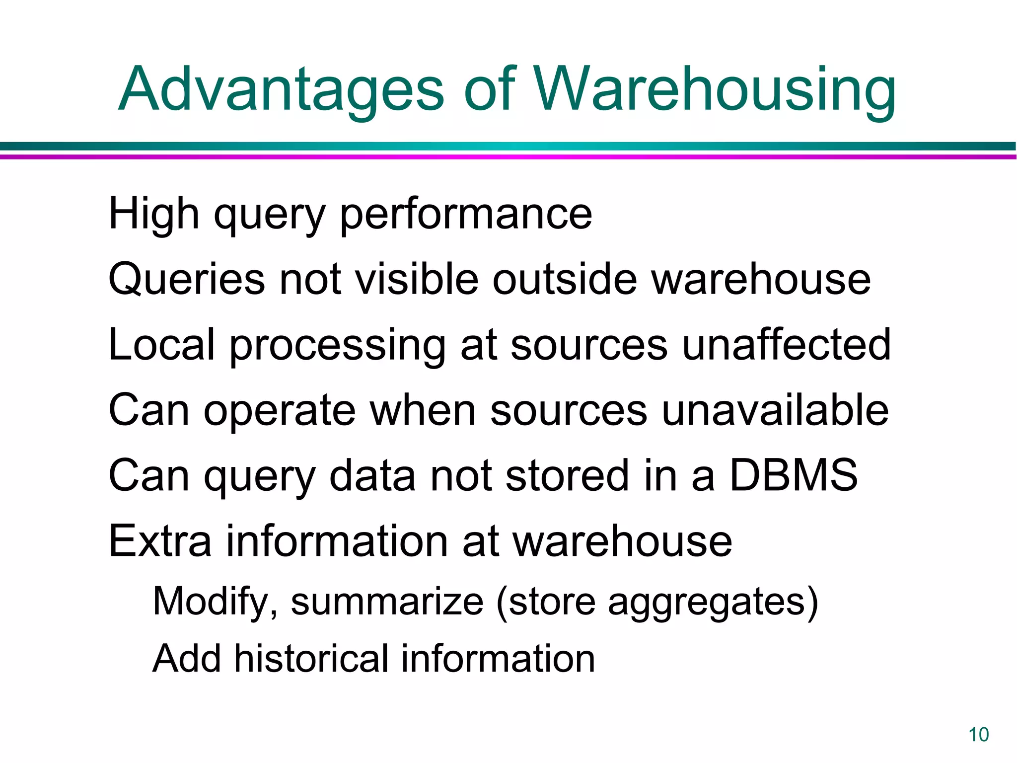
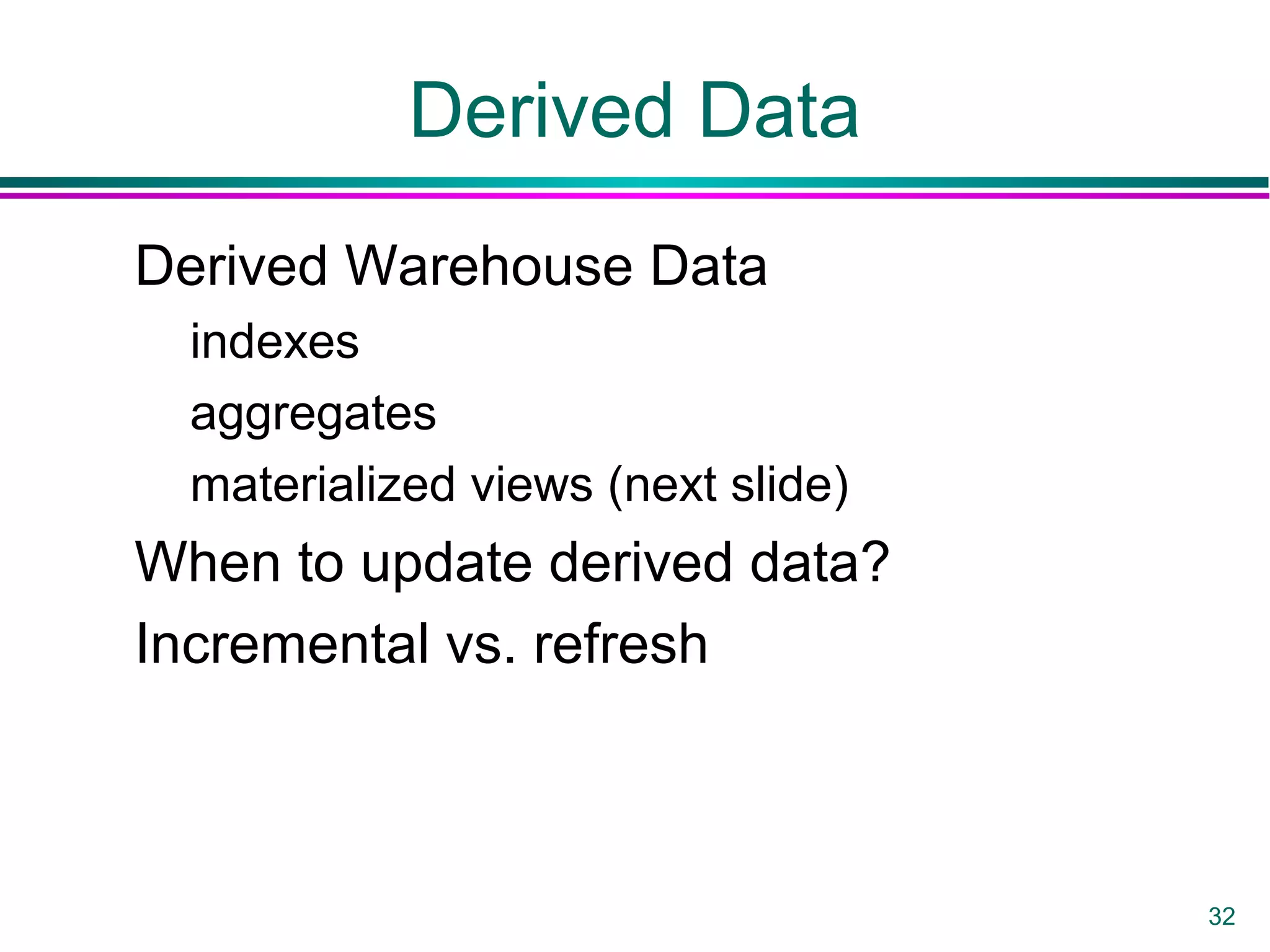
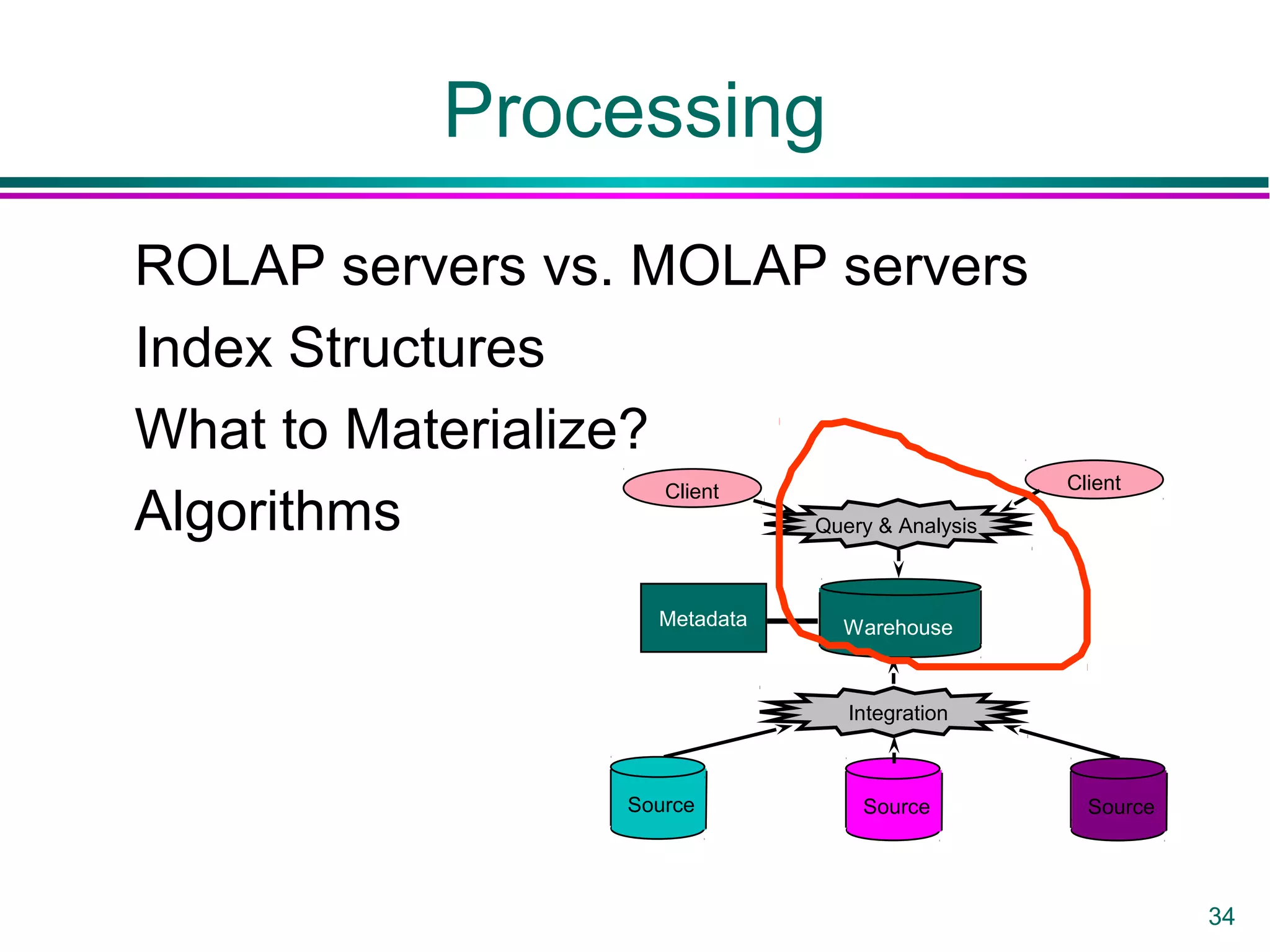
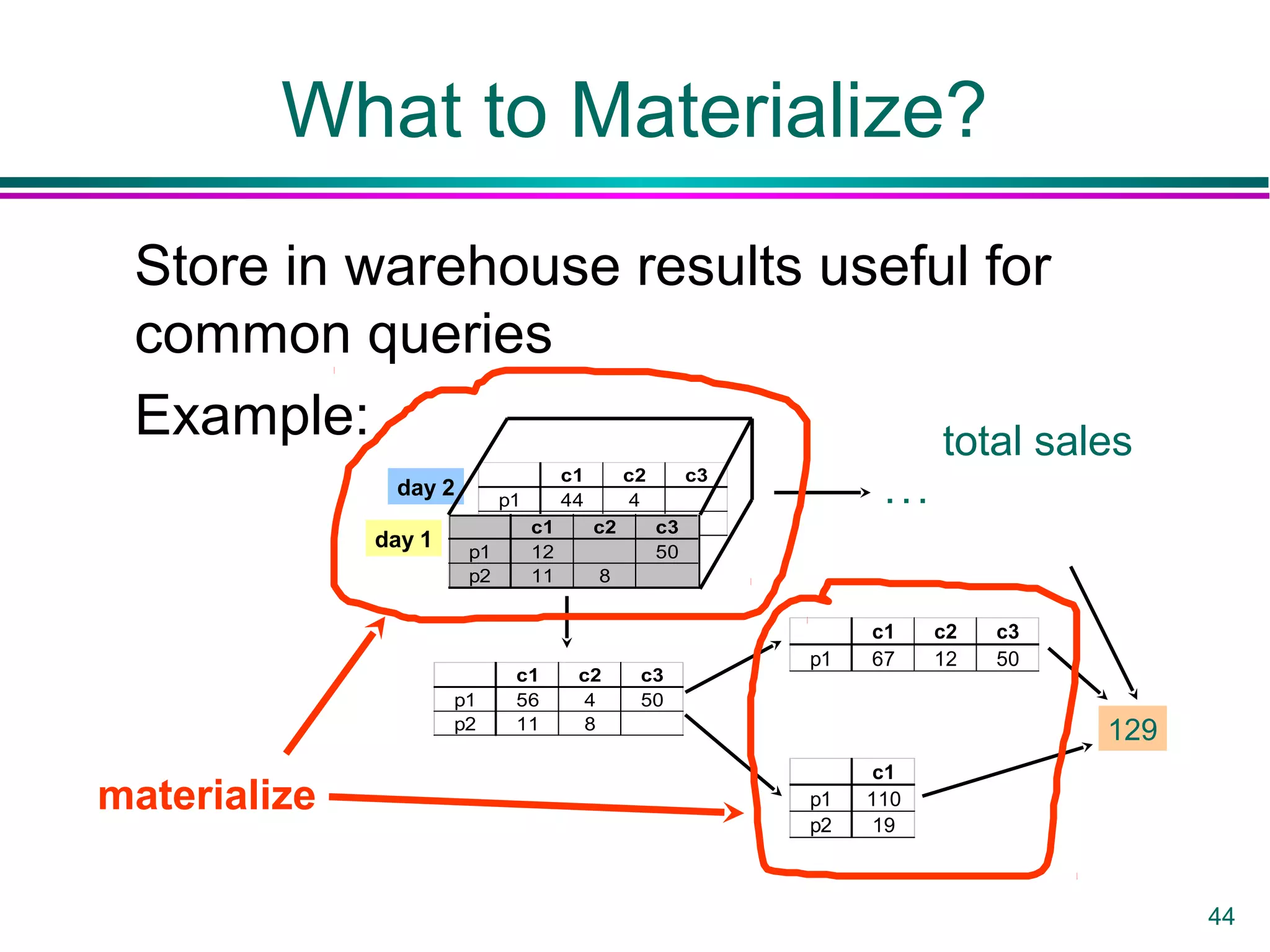
This document provides an overview of data warehousing. It defines a data warehouse as a collection of diverse data aimed at executives and decision makers that is integrated, time-varying, and non-volatile. It discusses why warehouses are used, different warehouse architectures and models, and operations like aggregation, pivoting and materializing views. Key benefits of warehouses include high query performance, flexibility to query data not in a DBMS, and ability to operate when sources are unavailable.

1. Data Warehousing
HEENA MADAN

2. 2
Warehousing
Growing industry: $8 billion way back in
1998
Range from desktop to huge:
Walmart: 900-CPU, 2,700 disk, 23TB
Teradata system
Lots of buzzwords, hype
slice & dice, rollup, MOLAP, pivot, ...

3. 3
Outline
What is a data warehouse?
Why a warehouse?
Models & operations
Implementing a warehouse
Future directions

4. 4
What is a Warehouse?
Collection of diverse data
subject oriented
aimed at executive, decision maker
often a copy of operational data
with value-added data (e.g., summaries, history)
integrated
time-varying
non-volatile
more

5. 5
What is a Warehouse?
Collection of tools
gathering data
cleansing, integrating, ...
querying, reporting, analysis
data mining
monitoring, administering warehouse

6. 6
Warehouse Architecture
Client Client
Warehouse
Source Source Source
Query & Analysis
Integration
Metadata

7. 7
Motivating Examples
Forecasting
Comparing performance of units
Monitoring, detecting fraud
Visualization

8. 8
Why a Warehouse?
Two Approaches:
Query-Driven (Lazy)
Warehouse (Eager)
Source Source
?

9. 9
Query-Driven Approach
Client Client
Wrapper Wrapper Wrapper
Mediator
Source Source Source

10. 10
Advantages of Warehousing
High query performance
Queries not visible outside warehouse
Local processing at sources unaffected
Can operate when sources unavailable
Can query data not stored in a DBMS
Extra information at warehouse
Modify, summarize (store aggregates)
Add historical information

11. 11
Advantages of Query-Driven
No need to copy data
less storage
no need to purchase data
More up-to-date data
Query needs can be unknown
Only query interface needed at sources
May be less draining on sources

12. 12
OLTP vs. OLAP
OLTP: On Line Transaction Processing
Describes processing at operational sites
OLAP: On Line Analytical Processing
Describes processing at warehouse

13. 13
OLTP vs. OLAP
Mostly updates
Many small transactions
Mb-Gb of data
Raw data
Clerical users
Up-to-date data
Consistency,
recoverability critical
Mostly reads
Queries long, complex
Gb-Tb of data
Summarized,
consolidated data
Decision-makers,
analysts as users
OLTP OLAP

14. 14
Data Marts
Smaller warehouses
Spans part of organization
e.g., marketing (customers, products, sales)
Do not require enterprise-wide consensus
but long term integration problems?

15. 15
Warehouse Models & Operators
Data Models
relations
stars & snowflakes
cubes
Operators
slice & dice
roll-up, drill down
pivoting
other

16. 16
Star
customer custId name address city
53 joe 10 main sfo
81 fred 12 main sfo
111 sally 80 willow la
product prodId name price
p1 bolt 10
p2 nut 5
store storeId city
c1 nyc
c2 sfo
c3 la
sale oderId date custId prodId storeId qty amt
o100 1/7/97 53 p1 c1 1 12
o102 2/7/97 53 p2 c1 2 11
105 3/8/97 111 p1 c3 5 50

17. 17
Star Schema
sale
orderId
date
custId
prodId
storeId
qty
amt
customer
custId
name
address
city
product
prodId
name
price
store
storeId
city

18. 18
Terms
Fact table
Dimension tables
Measures sale
orderId
date
custId
prodId
storeId
qty
amt
customer
custId
name
address
city
product
prodId
name
price
store
storeId
city

19. 19
Dimension Hierarchies
store storeId cityId tId mgr
s5 sfo t1 joe
s7 sfo t2 fred
s9 la t1 nancy
city cityId pop regId
sfo 1M north
la 5M south
region regId name
north cold region
south warm region
sType tId size location
t1 small downtown
t2 large suburbs
store
sType
city region
 snowflake schema
 constellations

20. 20
Cube
sale prodId storeId amt
p1 c1 12
p2 c1 11
p1 c3 50
p2 c2 8
c1 c2 c3
p1 12 50
p2 11 8
Fact table view:
Multi-dimensional cube:
dimensions = 2

21. 21
3-D Cube
sale prodId storeId date amt
p1 c1 1 12
p2 c1 1 11
p1 c3 1 50
p2 c2 1 8
p1 c1 2 44
p1 c2 2 4
day 2
c1 c2 c3
p1 44 4
p2 c1 c2 c3
p1 12 50
p2 11 8
day 1
dimensions = 3
Multi-dimensional cube:Fact table view:

22. 22
ROLAP vs. MOLAP
ROLAP:
Relational On-Line Analytical Processing
MOLAP:
Multi-Dimensional On-Line Analytical
Processing

23. 23
Aggregates
sale prodId storeId date amt
p1 c1 1 12
p2 c1 1 11
p1 c3 1 50
p2 c2 1 8
p1 c1 2 44
p1 c2 2 4
• Add up amounts for day 1
• In SQL: SELECT sum(amt) FROM SALE
WHERE date = 1
81

24. 24
Aggregates
sale prodId storeId date amt
p1 c1 1 12
p2 c1 1 11
p1 c3 1 50
p2 c2 1 8
p1 c1 2 44
p1 c2 2 4
• Add up amounts by day
• In SQL: SELECT date, sum(amt) FROM SALE
GROUP BY date
ans date sum
1 81
2 48

25. 25
Another Example
sale prodId storeId date amt
p1 c1 1 12
p2 c1 1 11
p1 c3 1 50
p2 c2 1 8
p1 c1 2 44
p1 c2 2 4
• Add up amounts by day, product
• In SQL: SELECT date, sum(amt) FROM SALE
GROUP BY date, prodId
sale prodId date amt
p1 1 62
p2 1 19
p1 2 48
drill-down
rollup

26. 26
Aggregates
Operators: sum, count, max, min,
median, ave
“Having” clause
Using dimension hierarchy
average by region (within store)
maximum by month (within date)

27. 27
Cube Aggregation
day 2
c1 c2 c3
p1 44 4
p2 c1 c2 c3
p1 12 50
p2 11 8
day 1
c1 c2 c3
p1 56 4 50
p2 11 8
c1 c2 c3
sum 67 12 50
sum
p1 110
p2 19
129
. . .
drill-down
rollup
Example: computing sums

28. 28
Cube Operators
day 2
c1 c2 c3
p1 44 4
p2 c1 c2 c3
p1 12 50
p2 11 8
day 1
c1 c2 c3
p1 56 4 50
p2 11 8
c1 c2 c3
sum 67 12 50
sum
p1 110
p2 19
129
. . .
sale(c1,*,*)
sale(*,*,*)
sale(c2,p2,*)

29. 29
c1 c2 c3 *
p1 56 4 50 110
p2 11 8 19
* 67 12 50 129
Extended Cube
day 2 c1 c2 c3 *
p1 44 4 48
p2
* 44 4 48
c1 c2 c3 *
p1 12 50 62
p2 11 8 19
* 23 8 50 81
day 1
*
sale(*,p2,*)

30. 30
Aggregation Using Hierarchies
day 2
c1 c2 c3
p1 44 4
p2 c1 c2 c3
p1 12 50
p2 11 8
day 1
region A region B
p1 56 54
p2 11 8
customer
region
country
(customer c1 in Region A;
customers c2, c3 in Region B)

31. 31
Pivoting
sale prodId storeId date amt
p1 c1 1 12
p2 c1 1 11
p1 c3 1 50
p2 c2 1 8
p1 c1 2 44
p1 c2 2 4
day 2
c1 c2 c3
p1 44 4
p2 c1 c2 c3
p1 12 50
p2 11 8
day 1
Multi-dimensional cube:Fact table view:
c1 c2 c3
p1 56 4 50
p2 11 8
Pivot turns unique values from
one column into unique columns
in the output

32. 32
Derived Data
Derived Warehouse Data
indexes
aggregates
materialized views (next slide)
When to update derived data?
Incremental vs. refresh

33. 33
Materialized Views
Define new warehouse relations using
SQL expressions
sale prodId storeId date amt
p1 c1 1 12
p2 c1 1 11
p1 c3 1 50
p2 c2 1 8
p1 c1 2 44
p1 c2 2 4
product id name price
p1 bolt 10
p2 nut 5
joinTb prodId name price storeId date amt
p1 bolt 10 c1 1 12
p2 nut 5 c1 1 11
p1 bolt 10 c3 1 50
p2 nut 5 c2 1 8
p1 bolt 10 c1 2 44
p1 bolt 10 c2 2 4
does not exist
at any source

34. 34
Processing
ROLAP servers vs. MOLAP servers
Index Structures
What to Materialize?
Algorithms
Client Client
Warehouse
Source Source Source
Query & Analysis
Integration
Metadata

35. 35
ROLAP Server
Relational OLAP Server
relational
DBMS
ROLAP
server
tools
utilities
sale prodId date sum
p1 1 62
p2 1 19
p1 2 48
Special indices, tuning;
Schema is “denormalized”

36. 36
MOLAP Server
Multi-Dimensional OLAP Server
multi-
dimensional
server
M.D. tools
utilities
could also
sit on
relational
DBMS
Product
City
Date
1 2 3 4
milk
soda
eggs
soap
A
B
Sales

37. 37
Index Structures
Traditional Access Methods
B-trees, hash tables, R-trees, grids, …
Popular in Warehouses
inverted lists
bit map indexes
join indexes
text indexes

38. 38
Inverted Lists
20
23
18
19
20
21
22
23
25
26
r4
r18
r34
r35
r5
r19
r37
r40
rId name age
r4 joe 20
r18 fred 20
r19 sally 21
r34 nancy 20
r35 tom 20
r36 pat 25
r5 dave 21
r41 jeff 26
...
age
index
inverted
lists
data
records

39. 39
Using Inverted Lists
Query:
Get people with age = 20 and name = “fred”
List for age = 20: r4, r18, r34, r35
List for name = “fred”: r18, r52
Answer is intersection: r18

40. 40
Bit Maps
20
23
18
19
20
21
22
23
25
26
id name age
1 joe 20
2 fred 20
3 sally 21
4 nancy 20
5 tom 20
6 pat 25
7 dave 21
8 jeff 26
...
age
index
bit
maps
data
records
1
1
0
1
1
0
0
0
0
0
0
1
0
0
0
1
0
1
1

41. 41
Using Bit Maps
Query:
Get people with age = 20 and name = “fred”
List for age = 20: 1101100000
List for name = “fred”: 0100000001
Answer is intersection: 010000000000
Good if domain cardinality small
Bit vectors can be compressed

42. 42
Join
sale prodId storeId date amt
p1 c1 1 12
p2 c1 1 11
p1 c3 1 50
p2 c2 1 8
p1 c1 2 44
p1 c2 2 4
• “Combine” SALE, PRODUCT relations
• In SQL: SELECT * FROM SALE, PRODUCT WHERE ...
product id name price
p1 bolt 10
p2 nut 5
joinTb prodId name price storeId date amt
p1 bolt 10 c1 1 12
p2 nut 5 c1 1 11
p1 bolt 10 c3 1 50
p2 nut 5 c2 1 8
p1 bolt 10 c1 2 44
p1 bolt 10 c2 2 4

43. 43
Join Indexes
product id name price jIndex
p1 bolt 10 r1,r3,r5,r6
p2 nut 5 r2,r4
sale rId prodId storeId date amt
r1 p1 c1 1 12
r2 p2 c1 1 11
r3 p1 c3 1 50
r4 p2 c2 1 8
r5 p1 c1 2 44
r6 p1 c2 2 4
join index

44. 44
What to Materialize?
Store in warehouse results useful for
common queries
Example:
day 2
c1 c2 c3
p1 44 4
p2 c1 c2 c3
p1 12 50
p2 11 8
day 1
c1 c2 c3
p1 56 4 50
p2 11 8
c1 c2 c3
p1 67 12 50
c1
p1 110
p2 19
129
. . .
total sales
materialize

45. 45
Materialization Factors
Type/frequency of queries
Query response time
Storage cost
Update cost

46. 46
Cube Aggregates Lattice
city, product, date
city, product city, date product, date
city product date
all
day 2
c1 c2 c3
p1 44 4
p2 c1 c2 c3
p1 12 50
p2 11 8
day 1
c1 c2 c3
p1 56 4 50
p2 11 8
c1 c2 c3
p1 67 12 50
129
use greedy
algorithm to
decide what
to materialize

47. 47
Dimension Hierarchies
all
state
city
cities city state
c1 CA
c2 NY

48. 48
Dimension Hierarchies
city, product
city, product, date
city, date product, date
city product date
all
state, product, date
state, date
state, product
state
not all arcs shown...

49. 49
Interesting Hierarchy
all
years
quarters
months
days
weeks
time day week month quarter year
1 1 1 1 2000
2 1 1 1 2000
3 1 1 1 2000
4 1 1 1 2000
5 1 1 1 2000
6 1 1 1 2000
7 1 1 1 2000
8 2 1 1 2000
conceptual
dimension table