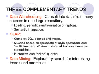
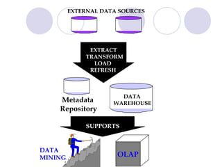
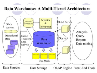
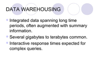
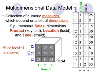
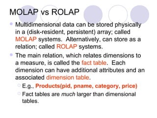
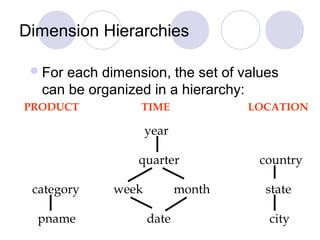
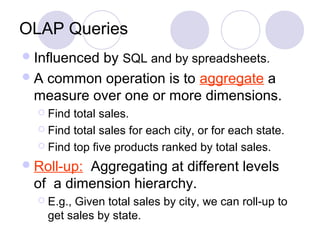
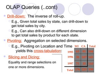
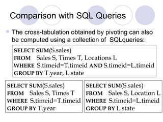
This document discusses data warehousing and online analytic processing (OLAP). It introduces key concepts such as data warehouses, OLAP, multidimensional data models, dimension hierarchies, and OLAP queries including roll-up, drill-down, pivoting, slicing and dicing. It also covers implementation issues such as indexing techniques and view maintenance to enable interactive queries for OLAP.

1. Data Warehouse & OLAP
Kuliah 1 Introduction
Slide banyak mengambil dari acuan-
acuan yang dipakai

2. DB, DW, DM
DW vs DB
DW vs DM

3. INTRODUCTION
Increasingly, organizations are analyzing
current and historical data to identify
useful patterns and support business
strategies.
Emphasis is on complex, interactive,
exploratory analysis of very large datasets
created by integrating data from across all
parts of an enterprise; data is fairly static.

4. INTRODUCTION (..cont)
Contrast such On-Line Analytic
Processing (OLAP) with traditional On-line
Transaction Processing (OLTP): mostly
long queries, instead of short update
transactions.
OLTP: roda penggerak organisasi
OLAP: mengawasi gerak roda
Cat: rencana mata kuliah transaction processing

5. THREE COMPLEMENTARY TRENDS
 Data Warehousing: Consolidate data from many
sources in one large repository.
 Loading, periodic synchronization of replicas.
 Semantic integration.
 OLAP:
 Complex SQL queries and views.
 Queries based on spreadsheet-style operations and
“multidimensional” view of data.  bahkan memakai
spreadsheet.
 Interactive and “online” queries.
 Data Mining: Exploratory search for interesting
trends and anomalies.

6. EXTERNAL DATA SOURCES
EXTRACT
TRANSFORM
LOAD
REFRESH
DATA
WAREHOUSEMetadata
Repository
SUPPORTS
OLAP
DATA
MINING

7. Data Warehouse: A Multi-Tiered ArchitectureData Warehouse: A Multi-Tiered Architecture
Data
Warehouse
Extract
Transform
Load
Refresh
OLAP Engine
Analysis
Query
Reports
Data mining
Monitor
&
Integrator
Metadata
Data Sources Front-End Tools
Serve
Data Marts
Operational
DBs
Other
sources
Data Storage
OLAP Server

8. DATA WAREHOUSING
Integrated data spanning long time
periods, often augmented with summary
information.
Several gigabytes to terabytes common.
Interactive response times expected for
complex queries.

9. Multidimensional Data Model
 Collection of numeric measures,
which depend on a set of dimensions.
 E.g., measure Sales, dimensions
Product (key: pid), Location (locid),
and Time (timeid).
8 10 10
30 20 50
25 8 15
1 2 3
timeid
pid
111213
11 1 1 25
11 2 1 8
11 3 1 15
12 1 1 30
12 2 1 20
12 3 1 50
13 1 1 8
13 2 1 10
13 3 1 10
11 1 2 35
pid
timeid
locid
sales
locid
Slice locid=1
is shown:

10. MOLAP vs ROLAP
 Multidimensional data can be stored physically
in a (disk-resident, persistent) array; called
MOLAP systems. Alternatively, can store as a
relation; called ROLAP systems.
 The main relation, which relates dimensions to
a measure, is called the fact table. Each
dimension can have additional attributes and an
associated dimension table.
 E.g., Products(pid, pname, category, price)
 Fact tables are much larger than dimensional
tables.

11. Dimension Hierarchies
For each dimension, the set of values
can be organized in a hierarchy:
PRODUCT TIME LOCATION
category week month state
pname date city
year
quarter country

12. OLAP Queries
Influenced by SQL and by spreadsheets.
A common operation is to aggregate a
measure over one or more dimensions.
 Find total sales.
 Find total sales for each city, or for each state.
 Find top five products ranked by total sales.
Roll-up: Aggregating at different levels
of a dimension hierarchy.
 E.g., Given total sales by city, we can roll-up to
get sales by state.

13. OLAP Queries (..cont)
 Drill-down: The inverse of roll-up.
 E.g., Given total sales by state, can drill-down to
get total sales by city.
 E.g., Can also drill-down on different dimension
to get total sales by product for each state.
 Pivoting: Aggregation on selected dimensions.
 E.g., Pivoting on Location and Time
yields this cross-tabulation:
 Slicing and Dicing:
Equality and range selections on
one or more dimensions.
63 81 144
38 107 145
75 35 110
WI CA Total
1995
1996
1997
176 223 339Total

14. Comparison with SQL Queries
 The cross-tabulation obtained by pivoting can also
be computed using a collection of SQLqueries:
SELECT SUM(S.sales)
FROM Sales S, Times T, Locations L
WHERE S.timeid=T.timeid AND S.timeid=L.timeid
GROUP BY T.year, L.state
SELECT SUM(S.sales)
FROM Sales S, Times T
WHERE S.timeid=T.timeid
GROUP BY T.year
SELECT SUM(S.sales)
FROM Sales S, Location L
WHERE S.timeid=L.timeid
GROUP BY L.state

15. The CUBE Operator
 Generalizing the previous example, if there
are k dimensions, we have 2^k possible SQL
GROUP BY queries that can be generated
through pivoting on a subset of dimensions.
 CUBE pid, locid, timeid BY SUM Sales
 Equivalent to rolling up Sales on all eight
subsets of the set {pid, locid, timeid}; each roll-
up corresponds to an SQL query of the form:
SELECT SUM(S.sales)
FROM Sales S
GROUP BY grouping-list
Lots of recent work on
optimizing the CUBE operator!

16. Design Issues
 Fact table in BCNF; dimension tables not
normalized.
 Dimension tables are small; updates/inserts/deletes are
rare. So, anomalies less important than good query
performance.
 This kind of schema is very common in OLAP
applications, and is called a star schema; computing
the join of all these relations is called a star join.
pricecategorypnamepid countrystatecitylocid
saleslocidtimeidpid
holiday_flagweekdatetimeid month quarter year
(Fact table)SALES
TIMES
PRODUCTS LOCATIONS

17. Implementation Issues
 New indexing techniques: Bitmap indexes, Join
indexes, array representations, compression,
precomputation of aggregations, etc.
 E.g., Bitmap index:
10
10
01
10
112 Joe M 3
115 Ram M 5
119 Sue F 5
112 Woo M 4
00100
00001
00001
00010
sex custid name sex rating ratingBit-vector:
1 bit for each
possible value.
Many queries can
be answered using
bit-vector ops!
M
F

18. Views and Decision Support
 OLAP queries are typically aggregate queries.
 Precomputation is essential for interactive response
times.
 The CUBE is in fact a collection of aggregate queries,
and precomputation is especially important: lots of
work on what is best to precompute given a limited
amount of space to store precomputed results.
 Warehouses can be thought of as a collection of
asynchronously replicated tables and periodically
maintained views.
 Has renewed interest in view maintenance!

19. View Modification (Evaluate On Demand)
CREATE VIEW RegionalSales(category,sales,state)
AS SELECT P.category, S.sales, L.state
FROM Products P, Sales S, Locations L
WHERE P.pid=S.pid AND S.locid=L.locid
SELECT R.category, R.state, SUM(R.sales)
FROM RegionalSales AS R GROUP BY R.category, R.state
SELECT R.category, R.state, SUM(R.sales)
FROM (SELECT P.category, S.sales, L.state
FROM Products P, Sales S, Locations L
WHERE P.pid=S.pid AND S.locid=L.locid) AS R
GROUP BY R.category, R.state
View
Query
Modified
Query

20. Interactive Queries
 Top N Queries: If you want to find the 10 (or
so) cheapest cars, it would be nice if the DB
could avoid computing the costs of all cars
before sorting to determine the 10 cheapest.
 Idea: Guess at a cost c such that the 10 cheapest all
cost less than c, and that not too many more cost
less. Then add the selection cost<c and evaluate
the query.
 If the guess is right, great, we avoid computation
for cars that cost more than c.
 If the guess is wrong, need to reset the selection
and recompute the original query.

21. Top N Queries
SELECT P.pid, P.pname, S.sales
FROM Sales S, Products P
WHERE S.pid=P.pid AND S.locid=1 AND S.timeid=3
ORDER BY S.sales DESC
OPTIMIZE FOR 10 ROWS
 OPTIMIZE FOR construct is not in SQL:1999!
 Cut-off value c is chosen by optimizer.
SELECT P.pid, P.pname, S.sales
FROM Sales S, Products P
WHERE S.pid=P.pid AND S.locid=1 AND S.timeid=3
AND S.sales > c
ORDER BY S.sales DESC

22. Interactive Queries
Online Aggregation: Consider an
aggregate query, e.g., finding the average
sales by state. Can we provide the user
with some information before the exact
average is computed for all states?