Download to read offline


![What is Data Warehouse?What is Data Warehouse?
• “A data warehouse is a subject-oriented, integrated,
time-variant, and nonvolatile collection of data in
support of management’s decision-making
process.”—W. H. Inmon
• A Data Warehouse is used for On-Line-Analytical-
Processing:
“Class of tools that enables the user to gain insight into data through interactive
access to a wide variety of possible views of the information”
• 3 Billion market worldwide [1999 figure,
olapreport.com]
o Retail industries: user profiling, inventory management
o Financial services: credit card analysis, fraud detection
o Telecommunications: call analysis, fraud detection](https://image.slidesharecdn.com/datawarehousingolapppt-3-160506122153/85/Data-ware-housing-Introduction-to-olap-3-320.jpg)
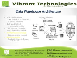

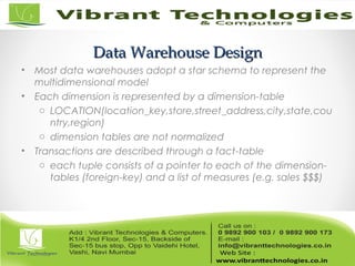


![Other Extensions to SQLOther Extensions to SQL
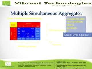
• Complex aggregation at multiple granularities (Ross et. all 1998)
o Compute multiple dependent aggregates
• Other proposals: the MD-join operator (Chatziantoniou et. all 1999]
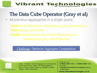
SELECT LOCATION.store, SALES.product_key, SUM (amount)
FROM SALES, LOCATION
WHERE SALES.location_key=LOCATION.location_key
CUBE BY SALES.product_key, LOCATION.store: R
SUCH THAT R.amount = max(amount)](https://image.slidesharecdn.com/datawarehousingolapppt-3-160506122153/85/Data-ware-housing-Introduction-to-olap-25-320.jpg)


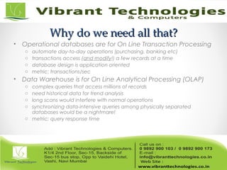
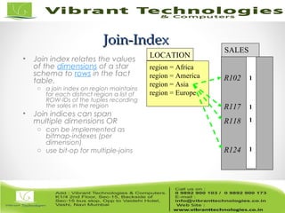
![View Selection ProblemView Selection Problem
• Selection is based on a workload estimate (e.g. logs) and a
given constraint (disk space or update window)
• NP-hard, optimal selection can not be computed > 4-5
dimensions
o greedy algorithms (e.g. [Harinarayan96]) run at least in polynomial
time in the number of views i.e exponential in the number of
dimensions!!!
• Optimal selection can not be approximated [Karloff99]
o greedy view selection can behave arbitrary bad
• Lack of good models for a cost-based optimization!](https://image.slidesharecdn.com/datawarehousingolapppt-3-160506122153/85/Data-ware-housing-Introduction-to-olap-31-320.jpg)


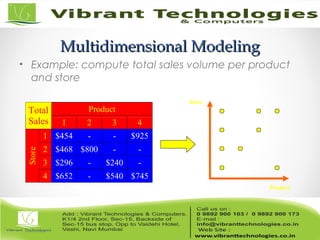
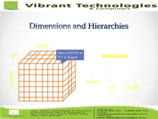
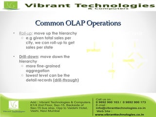
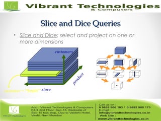
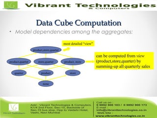
The document provides an overview of data warehousing, defining it as an integrated and non-volatile collection of data designed to support decision-making through online analytical processing (OLAP). It discusses the architecture of data warehouses, key concepts like star schemas, multidimensional modeling, and OLAP operations, while highlighting the differences between operational databases and data warehouses. The document also covers issues related to data cube computation, index usage, and explores the challenges of optimizing aggregate queries in complex multidimensional data environments.


![5G Explained! A High Level Overview [Introduction]](https://cdn.slidesharecdn.com/ss_thumbnails/5gexplainedahighleveloverview-260119165306-cc137a3e-thumbnail.jpg?width=640&height=640&fit=bounds)


