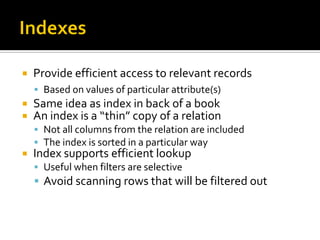
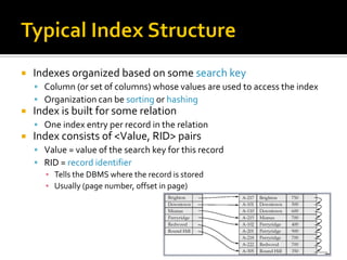
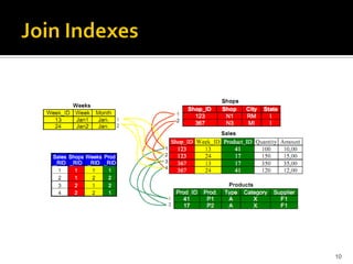
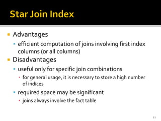
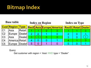
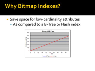
DATA WAREHOUSING
Physical Design
2
   Provide efficient access to relevant records
     Based on values of particular attribute(s)
   Same idea as index in back of a book
   An index is a “thin” copy of a relation
     Not all columns from the relation are included
     The index is sorted in a particular way
   Index supports efficient lookup
     Useful when filters are selective
     Avoid scanning rows that will be filtered out
   Indexes organized based on some search key
     Column (or set of columns) whose values are used to access the index
     Organization can be sorting or hashing
   Index is built for some relation
     One index entry per record in the relation
   Index consists of <Value, RID> pairs
     Value = value of the search key for this record
     RID = record identifier
      ▪ Tells the DBMS where the record is stored
      ▪ Usually (page number, offset in page)
   Traditional Access Methods
     B-trees, hash tables, R-trees, grids, …
   Popular in Warehouses
     Covering indexes
     Multi column indexes
     join indexes
     bit map indexes


                                                5
   Idea behind fact index:
     Thinner version of fact table
     Index takes up less space than fact table
     Fewer I/Os required to scan it
   Index has 1 index entry per fact table row
     Regardless of how many columns are in the
      index
   Sometimes an index has all the data you need
     Allows index-only query plan
     Not necessary to access the actual tuples
     Such an index is called a covering index

   SELECT COUNT(*) FROM R WHERE A=5
     Use index on A
     Count number of <5,RID> entries
     No need to look up records referenced by RIDs
   Multi-column indexes are very useful in data warehousing
     We say such an index has a composite key
   Example: B-Tree index on (A,B)
       Search key is (A,B) combination
       Index entries sorted by A value
       Entries with same A value are sorted by B value
       Called a lexicographic sort
   SELECT SUM(B) FROM R WHERE A=5
     Our (A,B) index covers this query!
   Coverage vs. size trade-off
     More attributes in search key → index covers more queries
     More attributes in search key → index takes up more disk space
10
   Advantages
     efficient computation of joins involving first index
      columns (or all columns)
   Disadvantages
     useful only for specific join combinations
      ▪ for general usage, it is necessary to store a high number
        of indices
     required space may be significant
      ▪ joins always involve the fact table


                                                                    11
Base table              Index on Region                  Index on Type
Cust   Region    Type RecIDAsia Europe America RecID Retail Dealer
C1     Asia      Retail 1   1     0      0       1     1      0
C2     Europe    Dealer 2   0     1      0       2     0      1
C3     Asia      Dealer 3   1     0      0       3     0      1
C4     America   Retail 4   0     0      1       4     1      0
C5     Europe    Dealer 5   0     1      0       5     0      1

       Query:
          Get customer with region = „Asia‟ AND type = “Dealer”


                                                                           12
   Good if domain cardinality small
     Most useful for attributes with low or
      medium cardinality
      ▪ Not good for something like LastName


                                               13
   Index intersection plans with bitmap indexes
    are fast
     Just perform bitwise AND!
     Index intersection with B-Trees requires a
      join
   Save space for low-cardinality attributes
     As compared to a B-Tree or Hash index
   Bit vectors can be compressed
   Compression Pros and Cons
     Reduce storage space → reduce number of I/Os required
     Need to compress/uncompress → increase CPU work
      required
     Each compression scheme negotiates this trade-off
      differently
     Operate directly on compressed bitmap → improved
      performance


                                                              16
   Bit matrix which precomputes the join between a
    dimension and the fact table
     one column for each dimension RID
     one row for each fact table RID
     cell (i,j) is 1 if fact table tuple i joins dimension tuple j, 0
      otherwise
   Indexing dimensions
     attributes frequently involved in selection predicates
     if domain cardinality is high, then B-tree index
     if domain cardinality is low, then bitmap index
   Indices for join
     indexing only foreign keys in the fact table is rarely
      appropriate
     star join index should be used with caution (column order
      issue)
     bitmapped join index is suggested (if available)
   Indices for group by
     use materialized views

Diseño fisico indices_2

  • 1.
  • 2.
  • 3.
    Provide efficient access to relevant records  Based on values of particular attribute(s)  Same idea as index in back of a book  An index is a “thin” copy of a relation  Not all columns from the relation are included  The index is sorted in a particular way  Index supports efficient lookup  Useful when filters are selective  Avoid scanning rows that will be filtered out
  • 4.
    Indexes organized based on some search key  Column (or set of columns) whose values are used to access the index  Organization can be sorting or hashing  Index is built for some relation  One index entry per record in the relation  Index consists of <Value, RID> pairs  Value = value of the search key for this record  RID = record identifier ▪ Tells the DBMS where the record is stored ▪ Usually (page number, offset in page)
  • 5.
    Traditional Access Methods  B-trees, hash tables, R-trees, grids, …  Popular in Warehouses  Covering indexes  Multi column indexes  join indexes  bit map indexes 5
  • 6.
    Idea behind fact index:  Thinner version of fact table  Index takes up less space than fact table  Fewer I/Os required to scan it
  • 7.
    Index has 1 index entry per fact table row  Regardless of how many columns are in the index
  • 8.
    Sometimes an index has all the data you need  Allows index-only query plan  Not necessary to access the actual tuples  Such an index is called a covering index  SELECT COUNT(*) FROM R WHERE A=5  Use index on A  Count number of <5,RID> entries  No need to look up records referenced by RIDs
  • 9.
    Multi-column indexes are very useful in data warehousing  We say such an index has a composite key  Example: B-Tree index on (A,B)  Search key is (A,B) combination  Index entries sorted by A value  Entries with same A value are sorted by B value  Called a lexicographic sort  SELECT SUM(B) FROM R WHERE A=5  Our (A,B) index covers this query!  Coverage vs. size trade-off  More attributes in search key → index covers more queries  More attributes in search key → index takes up more disk space
  • 10.
  • 11.
    Advantages  efficient computation of joins involving first index columns (or all columns)  Disadvantages  useful only for specific join combinations ▪ for general usage, it is necessary to store a high number of indices  required space may be significant ▪ joins always involve the fact table 11
  • 12.
    Base table Index on Region Index on Type Cust Region Type RecIDAsia Europe America RecID Retail Dealer C1 Asia Retail 1 1 0 0 1 1 0 C2 Europe Dealer 2 0 1 0 2 0 1 C3 Asia Dealer 3 1 0 0 3 0 1 C4 America Retail 4 0 0 1 4 1 0 C5 Europe Dealer 5 0 1 0 5 0 1 Query: Get customer with region = „Asia‟ AND type = “Dealer” 12
  • 13.
    Good if domain cardinality small  Most useful for attributes with low or medium cardinality ▪ Not good for something like LastName 13
  • 14.
    Index intersection plans with bitmap indexes are fast  Just perform bitwise AND!  Index intersection with B-Trees requires a join
  • 15.
    Save space for low-cardinality attributes  As compared to a B-Tree or Hash index
  • 16.
    Bit vectors can be compressed  Compression Pros and Cons  Reduce storage space → reduce number of I/Os required  Need to compress/uncompress → increase CPU work required  Each compression scheme negotiates this trade-off differently  Operate directly on compressed bitmap → improved performance 16
  • 17.
    Bit matrix which precomputes the join between a dimension and the fact table  one column for each dimension RID  one row for each fact table RID  cell (i,j) is 1 if fact table tuple i joins dimension tuple j, 0 otherwise
  • 18.
    Indexing dimensions  attributes frequently involved in selection predicates  if domain cardinality is high, then B-tree index  if domain cardinality is low, then bitmap index  Indices for join  indexing only foreign keys in the fact table is rarely appropriate  star join index should be used with caution (column order issue)  bitmapped join index is suggested (if available)  Indices for group by  use materialized views