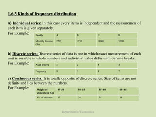
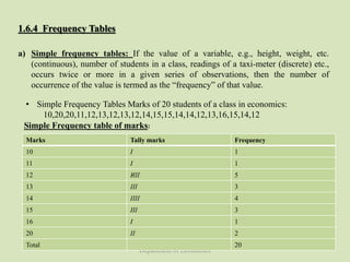
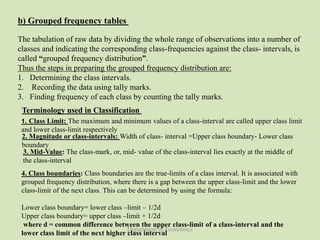
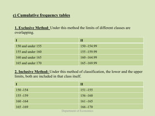
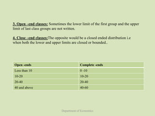
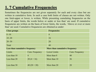
ECONOMICS
BASIC
STATISTICS
Dr Rekha Choudhary
Department of Economics
Jai NarainVyas University,Jodhpur
Rajasthan
Department of Economics
Classification
Data
Data
Data
Data
1.0 Introduction
Data Presentation
The objective of classification of
data is to make the data simple ,
concise, meaningful and interesting
and helpful in further analysis.
Department of Economics
1.1 Objectives
After going through this unit, you will
be able to understand:
 Need of Classification;
 Classification of Data;
 Characteristics of Classification
 Terminology used in Quantitative
Classification, and
 Frequency and Frequency
distribution
Department of Economics
1.2 Need of Classification
 The raw data collected through surveys or experiments will be of no use if it
is haphazard and unsystematic
 Because that data is not appropriate to draw conclusions and make
interpretations
 Hence it becomes important to arrange data into a systematic form so as to
identify the number of units belongings to a particular classified group.
Department of Economics
1.3 Classification
1.3.1 Meaning of Classification
The placement of data in different homogenous groups formed on the basis of some
characteristics or criteria is called classification
1.3.2 Definition of Economists
According to L. R Connor
“Classification is the process of arranging things (actually or notionally) in groups or
classes according to their resemblance and affinities, and gives expression to the unity of
attributes that may subsist amongst the diversity of individuals”.
According to J. R Hicks
“Classification and arranged facts speak themselves, unarranged they are as dead as
mutton”
Department of Economics
1.3.3 Characteristics of Classification
 Data Classification
 Homogeneity in diversity
 Actually or/ notionally
1.3.4 Objectives of Classification
 Easy and concise
 Homogeneity
 Helps to compare
 Mutually relative
 Scientific arrangements
 Basis of Tabulation
Department of Economics
1.4 Basis of Classification
In the process of tabulation the following type of classification are encountered
1. Geographical Classification: Data are arranged according to place, areas or region.
2. Chronological or time Classification: Data is arranged according to time i.e. weekly,
monthly, quarterly, half yearly, annually etc.
3. Qualitative Classification: Data are arranged according to the attributes like sex, marital
status, educational status, stage or intensity of disease
4. Quantitative Classification: Means arranging data according to certain characteristics
that can be measured e.g. height, weight or income of person etc.
H. A, Struger suggested a formula to determine approximate class interval and
number of classes as follow:
Where, L= largest observation
S= smallest Observation
I = class interval
n = total number of observation
i = L – S
1 + 3.322 log N
Department of Economics
1.5 Frequency
Number of times variables value is repeated is called Frequency. Suppose 50 women
working in the college, in this 50 frequency is the women working in the college
1.5.1 Frequency Array
When the individual items or values of the variable are given along, with their
corresponding frequencies, it is know as Frequency array.
The education level of men is presented as below:
Education
level
Up to primary
level
Up to
secondary
level
Up to
graduation
level
Up to post
graduation
level
No. of Men 70 15 20 10
Note: This presentation of data is know as Frequency array
Department of Economics
1.6 Frequency Distribution
1.6.1 Definition
• Tally bars are used for used for arrangement of frequencies in different groups
• Frequency distribution gives a better picture of the pattern of data if the number of
items is large enough.
• From a frequency array, it is not possible to compare characteristics of different
groups.
1.6.2 The basic factors of frequency distribution are:
i) Variable
ii) Frequency
Variable: Those numerical characteristics, the measurement of which is different for
different persons and which fluctuate in quantity or size are called variables.
Variables can be two types:
• Discrete variable
• Continuous variable
Department of Economics
1.6.3 Kinds of frequency distribution
a) Individual series: In this case every items is independent and the measurement of
each item is given separately.
For Example:
b) Discrete series: Discrete series of data is one in which exact measurement of each
unit is possible in whole numbers and individual value differ with definite breaks.
For Example:
c) Continuous series: It is totally opposite of discrete series. Size of items are not
definite and lies between the numbers.
For Example:
Family A B C D
Monthly Income
(Rs)
2500 1750 18000 5000
No of letters 1 2 3 4
Frequency 9 5 4 7
Weight of
students(in Kg)
45 -50 50 -55 55 -60 60 -65
No. of students 12 28 35 18
Department of Economics
1.6.4 Frequency Tables
a) Simple frequency tables: If the value of a variable, e.g., height, weight, etc.
(continuous), number of students in a class, readings of a taxi-meter (discrete) etc.,
occurs twice or more in a given series of observations, then the number of
occurrence of the value is termed as the “frequency” of that value.
• Simple Frequency Tables Marks of 20 students of a class in economics:
10,20,20,11,12,13,12,13,12,14,15,15,14,14,12,13,16,15,14,12
Marks Tally marks Frequency
10 I 1
11 I 1
12 I̷III 5
13 III 3
14 IIII 4
15 III 3
16 I 1
20 II 2
Total 20
Simple Frequency table of marks:
Department of Economics
b) Grouped frequency tables
The tabulation of raw data by dividing the whole range of observations into a number of
classes and indicating the corresponding class-frequencies against the class- intervals, is
called “grouped frequency distribution”.
Thus the steps in preparing the grouped frequency distribution are:
1. Determining the class intervals.
2. Recording the data using tally marks.
3. Finding frequency of each class by counting the tally marks.
Terminology used in Classification
1. Class Limit: The maximum and minimum values of a class-interval are called upper class limit
and lower class-limit respectively
2. Magnitude or class-intervals: Width of class- interval =Upper class boundary- Lower class
boundary
3. Mid-Value: The class-mark, or, mid- value of the class-interval lies exactly at the middle of
the class-interval
4. Class boundaries: Class boundaries are the true-limits of a class interval. It is associated with
grouped frequency distribution, where there is a gap between the upper class-limit and the lower
class-limit of the next class. This can be determined by using the formula:
Lower class boundary= lower class –limit – 1/2d
Upper class boundary= upper class –limit + 1/2d
where d = common difference between the upper class-limit of a class-interval and the
lower class limit of the next higher class interval
Department of Economics
1. Exclusive Method: Under this method the limits of different classes are
overlapping.
2. Inclusive Method: Under this method of classification, the lower and the upper
limits, both are included in that class itself.
I II
150 and under 155 150 -154.99
155 and under 160 155 -159.99
160 and under 165 160 -164.99
165 and under 170 165 -169.99
I II
150 -154 151 -155
155 -159 156 -160
160 -164 161 -165
165 -169 166 -170
c) Cumulative frequency tables
Department of Economics
3. Open –end classes: Sometimes the lower limit of the first group and the upper
limit of last class groups are not written.
4. Close –end classes:The opposite would be a closed ended distribution i.e
when both the lower and upper limits are closed or bounded..
Open -ends Complete -ends
Less than 10 0 -10
10-20 10-20
20-40 20-40
40 and above 40-60
Department of Economics
1. 7 Cumulative Frequencies
Sometimes the frequencies are not given separately for each and every class but are
written in cumulative form. In such a case both limits of classes are not written. Only
one limit-upper or lower, is written. While presenting cumulating frequencies on the
basis of upper limits, the words below or under or less than’ are used. If cumulative
frequencies are written on the basis of lower limits, the words, ‘Above or over or more
than’ are used. Cumulative frequencies are obtained as under:
Class groups Frequencies
0 -10 4
10 -20 16
20 -30 20
Total 40
Less than cumulative frequency More than cumulative frequency
Limits Cum. Frequency Lower Limits Cum. Frequency
Less than 10 4 More than 0 40
Less than 20 20 (4 + 16) More than 10 36
Less than 30 40 (20 + 20) More than 20 20
Department of Economics
1.8 Let us Sum up
In present era people must have some knowledge of Data, how to collect data ,
what are the methods of collection of data with how to classify the data. So,
keeping that in mind after the study of this unit we know about classification
of data , need of data classification, method of classification of data,
frequencies distribution and concept of different series like induvial series,
discrete series and continuous series. As can be seen from the above discussion
that the objective of classification of data is to make the data simple , concise,
meaningful and interesting and helpful in further analysis. Hence it becomes
important to arrange data into a systematic form so as to identify the number of
units belongings to a particular classified group.
Department of Economics
1. Define Classification. Discuss the purpose and methods of classification
giving suitable examples.
2. Discuss the Main elements of an ideal classification.
3. Distinguish Between:
• Continuous series &Discrete series
• Exclusive &Inclusive series
4. Determine the magnitude and the number of classes
10.0, 10.6, 10.9, 11.8, 12.3, 11.6, 11.9, 10.3, 10.9, 12.3, 12.8, 10.4, 11.2,
10.7, 11.0, 11.1, 10.8, 12.5, 11.8, 12.0, 12.2
1.9 Unit End Questions
Department of Economics
1.10 Suggested Readings
Asthana H.S, and Bhushan, B.(2007) Statistics for Social Sciences (with SPSS
Applications). Prentice Hall of India
B.L.Aggrawal (2009). Basic Statistics. New Age International Publisher, Delhi.
Gupta, S.C.(1990) Fundamentals of Statistics. Himalaya Publishing House, Mumbai
Elhance, D.N: Fundamental of Statistics
Singhal, M.L: Elements of Statistics
Nagar, A.L. and Das, R.K.: Basic Statistics
Croxton Cowden: Applied General Statistics
Nagar, K.N.: Sankhyiki ke mool tatva
Gupta, BN : Sankhyiki
References
https://www.google.com/url?sa=i&url=https%3A%2F%2Fexaminer.pk%2Fdata-
classificationtabulation-and-presentation-online-
exam%2F&psig=AOvVaw22jc1fPDLPyvOMYDZaVo4a&ust=1596197303991000&source=images
&cd=vfe&ved=0CAIQjRxqFwoTCMiu1MD49OoCFQAAAAAdAAAAABAJ

Classification of data

  • 1.
    ECONOMICS BASIC STATISTICS Dr Rekha Choudhary Departmentof Economics Jai NarainVyas University,Jodhpur Rajasthan
  • 2.
    Department of Economics Classification Data Data Data Data 1.0Introduction Data Presentation The objective of classification of data is to make the data simple , concise, meaningful and interesting and helpful in further analysis.
  • 3.
    Department of Economics 1.1Objectives After going through this unit, you will be able to understand:  Need of Classification;  Classification of Data;  Characteristics of Classification  Terminology used in Quantitative Classification, and  Frequency and Frequency distribution
  • 4.
    Department of Economics 1.2Need of Classification  The raw data collected through surveys or experiments will be of no use if it is haphazard and unsystematic  Because that data is not appropriate to draw conclusions and make interpretations  Hence it becomes important to arrange data into a systematic form so as to identify the number of units belongings to a particular classified group.
  • 5.
    Department of Economics 1.3Classification 1.3.1 Meaning of Classification The placement of data in different homogenous groups formed on the basis of some characteristics or criteria is called classification 1.3.2 Definition of Economists According to L. R Connor “Classification is the process of arranging things (actually or notionally) in groups or classes according to their resemblance and affinities, and gives expression to the unity of attributes that may subsist amongst the diversity of individuals”. According to J. R Hicks “Classification and arranged facts speak themselves, unarranged they are as dead as mutton”
  • 6.
    Department of Economics 1.3.3Characteristics of Classification  Data Classification  Homogeneity in diversity  Actually or/ notionally 1.3.4 Objectives of Classification  Easy and concise  Homogeneity  Helps to compare  Mutually relative  Scientific arrangements  Basis of Tabulation
  • 7.
    Department of Economics 1.4Basis of Classification In the process of tabulation the following type of classification are encountered 1. Geographical Classification: Data are arranged according to place, areas or region. 2. Chronological or time Classification: Data is arranged according to time i.e. weekly, monthly, quarterly, half yearly, annually etc. 3. Qualitative Classification: Data are arranged according to the attributes like sex, marital status, educational status, stage or intensity of disease 4. Quantitative Classification: Means arranging data according to certain characteristics that can be measured e.g. height, weight or income of person etc. H. A, Struger suggested a formula to determine approximate class interval and number of classes as follow: Where, L= largest observation S= smallest Observation I = class interval n = total number of observation i = L – S 1 + 3.322 log N
  • 8.
    Department of Economics 1.5Frequency Number of times variables value is repeated is called Frequency. Suppose 50 women working in the college, in this 50 frequency is the women working in the college 1.5.1 Frequency Array When the individual items or values of the variable are given along, with their corresponding frequencies, it is know as Frequency array. The education level of men is presented as below: Education level Up to primary level Up to secondary level Up to graduation level Up to post graduation level No. of Men 70 15 20 10 Note: This presentation of data is know as Frequency array
  • 9.
    Department of Economics 1.6Frequency Distribution 1.6.1 Definition • Tally bars are used for used for arrangement of frequencies in different groups • Frequency distribution gives a better picture of the pattern of data if the number of items is large enough. • From a frequency array, it is not possible to compare characteristics of different groups. 1.6.2 The basic factors of frequency distribution are: i) Variable ii) Frequency Variable: Those numerical characteristics, the measurement of which is different for different persons and which fluctuate in quantity or size are called variables. Variables can be two types: • Discrete variable • Continuous variable
  • 10.
    Department of Economics 1.6.3Kinds of frequency distribution a) Individual series: In this case every items is independent and the measurement of each item is given separately. For Example: b) Discrete series: Discrete series of data is one in which exact measurement of each unit is possible in whole numbers and individual value differ with definite breaks. For Example: c) Continuous series: It is totally opposite of discrete series. Size of items are not definite and lies between the numbers. For Example: Family A B C D Monthly Income (Rs) 2500 1750 18000 5000 No of letters 1 2 3 4 Frequency 9 5 4 7 Weight of students(in Kg) 45 -50 50 -55 55 -60 60 -65 No. of students 12 28 35 18
  • 11.
    Department of Economics 1.6.4Frequency Tables a) Simple frequency tables: If the value of a variable, e.g., height, weight, etc. (continuous), number of students in a class, readings of a taxi-meter (discrete) etc., occurs twice or more in a given series of observations, then the number of occurrence of the value is termed as the “frequency” of that value. • Simple Frequency Tables Marks of 20 students of a class in economics: 10,20,20,11,12,13,12,13,12,14,15,15,14,14,12,13,16,15,14,12 Marks Tally marks Frequency 10 I 1 11 I 1 12 I̷III 5 13 III 3 14 IIII 4 15 III 3 16 I 1 20 II 2 Total 20 Simple Frequency table of marks:
  • 12.
    Department of Economics b)Grouped frequency tables The tabulation of raw data by dividing the whole range of observations into a number of classes and indicating the corresponding class-frequencies against the class- intervals, is called “grouped frequency distribution”. Thus the steps in preparing the grouped frequency distribution are: 1. Determining the class intervals. 2. Recording the data using tally marks. 3. Finding frequency of each class by counting the tally marks. Terminology used in Classification 1. Class Limit: The maximum and minimum values of a class-interval are called upper class limit and lower class-limit respectively 2. Magnitude or class-intervals: Width of class- interval =Upper class boundary- Lower class boundary 3. Mid-Value: The class-mark, or, mid- value of the class-interval lies exactly at the middle of the class-interval 4. Class boundaries: Class boundaries are the true-limits of a class interval. It is associated with grouped frequency distribution, where there is a gap between the upper class-limit and the lower class-limit of the next class. This can be determined by using the formula: Lower class boundary= lower class –limit – 1/2d Upper class boundary= upper class –limit + 1/2d where d = common difference between the upper class-limit of a class-interval and the lower class limit of the next higher class interval
  • 13.
    Department of Economics 1.Exclusive Method: Under this method the limits of different classes are overlapping. 2. Inclusive Method: Under this method of classification, the lower and the upper limits, both are included in that class itself. I II 150 and under 155 150 -154.99 155 and under 160 155 -159.99 160 and under 165 160 -164.99 165 and under 170 165 -169.99 I II 150 -154 151 -155 155 -159 156 -160 160 -164 161 -165 165 -169 166 -170 c) Cumulative frequency tables
  • 14.
    Department of Economics 3.Open –end classes: Sometimes the lower limit of the first group and the upper limit of last class groups are not written. 4. Close –end classes:The opposite would be a closed ended distribution i.e when both the lower and upper limits are closed or bounded.. Open -ends Complete -ends Less than 10 0 -10 10-20 10-20 20-40 20-40 40 and above 40-60
  • 15.
    Department of Economics 1.7 Cumulative Frequencies Sometimes the frequencies are not given separately for each and every class but are written in cumulative form. In such a case both limits of classes are not written. Only one limit-upper or lower, is written. While presenting cumulating frequencies on the basis of upper limits, the words below or under or less than’ are used. If cumulative frequencies are written on the basis of lower limits, the words, ‘Above or over or more than’ are used. Cumulative frequencies are obtained as under: Class groups Frequencies 0 -10 4 10 -20 16 20 -30 20 Total 40 Less than cumulative frequency More than cumulative frequency Limits Cum. Frequency Lower Limits Cum. Frequency Less than 10 4 More than 0 40 Less than 20 20 (4 + 16) More than 10 36 Less than 30 40 (20 + 20) More than 20 20
  • 16.
    Department of Economics 1.8Let us Sum up In present era people must have some knowledge of Data, how to collect data , what are the methods of collection of data with how to classify the data. So, keeping that in mind after the study of this unit we know about classification of data , need of data classification, method of classification of data, frequencies distribution and concept of different series like induvial series, discrete series and continuous series. As can be seen from the above discussion that the objective of classification of data is to make the data simple , concise, meaningful and interesting and helpful in further analysis. Hence it becomes important to arrange data into a systematic form so as to identify the number of units belongings to a particular classified group.
  • 17.
    Department of Economics 1.Define Classification. Discuss the purpose and methods of classification giving suitable examples. 2. Discuss the Main elements of an ideal classification. 3. Distinguish Between: • Continuous series &Discrete series • Exclusive &Inclusive series 4. Determine the magnitude and the number of classes 10.0, 10.6, 10.9, 11.8, 12.3, 11.6, 11.9, 10.3, 10.9, 12.3, 12.8, 10.4, 11.2, 10.7, 11.0, 11.1, 10.8, 12.5, 11.8, 12.0, 12.2 1.9 Unit End Questions
  • 18.
    Department of Economics 1.10Suggested Readings Asthana H.S, and Bhushan, B.(2007) Statistics for Social Sciences (with SPSS Applications). Prentice Hall of India B.L.Aggrawal (2009). Basic Statistics. New Age International Publisher, Delhi. Gupta, S.C.(1990) Fundamentals of Statistics. Himalaya Publishing House, Mumbai Elhance, D.N: Fundamental of Statistics Singhal, M.L: Elements of Statistics Nagar, A.L. and Das, R.K.: Basic Statistics Croxton Cowden: Applied General Statistics Nagar, K.N.: Sankhyiki ke mool tatva Gupta, BN : Sankhyiki References https://www.google.com/url?sa=i&url=https%3A%2F%2Fexaminer.pk%2Fdata- classificationtabulation-and-presentation-online- exam%2F&psig=AOvVaw22jc1fPDLPyvOMYDZaVo4a&ust=1596197303991000&source=images &cd=vfe&ved=0CAIQjRxqFwoTCMiu1MD49OoCFQAAAAAdAAAAABAJ