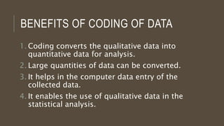
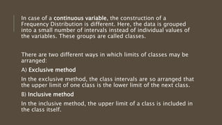
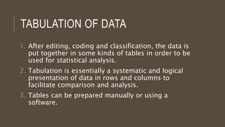
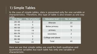
2. WHAT DOES PROCESSING OF DATA
MEAN?
oWhile conducting research, after the
collection of data is over, more often than
not the data obtained is quite raw and
unusable directly.
oProcessing required
oThis is possible only through systematic
processing of data.
3. STEPS INVOLVED IN PROCESSING
OF DATA
1) Editing
2) Coding
3) Classification
4) Tabulation
4. EDITING OF DATA
oEditing is the first stage in the processing
of data.
oEditing may be broadly defined to be a
procedure, which uses available
information and assumptions to substitute
inconsistent values in a data set.
oAccurate and complete data is the
requirement.
5. SOME GUIDELINES TO EDIT THE
DATA
1. A copy of the instructions for the interviewees
2. The editor should not destroy or erase the
original entry.
3. Clear edit indication required.
4. All completed schedules should have the
signature of the editor and the date.
6. SOME RULES FOR EDITING DATA
INCORRECT ANSWERS
1. It is quite common to get incorrect answers to many of the
questions. A person with a thorough knowledge will be able to
notice them.
2. Changes may be made if one is absolutely sure, else avoid.
3. Usually an entry has a number of questions and although answers
to a few questions are incorrect, it is advisable to use the other
correct information from the entry rather than discarding the
schedule entirely.
7. INCONSISTENT ANSWERS
1. If and when there are inconsistencies in the answers or when there
are incomplete or missing answers, the questionnaire should not
be used.
MODIFIED ANSWERS
1. Sometimes it may be necessary to modify or qualify the answers to
favor the research.
2. They have to be indicated for reference and checking.
3. For example, numerical answers are to be converted to same units.
8. CODING OF DATA
oCoding is basically a solution to the data entry
issue of research. It’s the process of converting
qualitative data into quantitative data.
oCoding refers to the process by which data is
categorized into groups and numerals or other
symbols or both are assigned to each item
depending on the class it falls in.
9. TYPES OF CODING
PRE-CODING
1.Precoding is the process of assigning the
codes to the attributes if the variable
before collecting the data.
POST-CODING
1.Post-coding is the process of assigning
the codes after the data collection.
10. BENEFITS OF CODING OF DATA
1. Coding converts the qualitative data into
quantitative data for analysis.
2. Large quantities of data can be converted.
3. It helps in the computer data entry of the
collected data.
4. It enables the use of qualitative data in the
statistical analysis.
11. CLASSIFICATION OF DATA
oAfter the data is collected and edited, the next step towards further
processing the data is classification.
oGenerally when the data is collected its heterogeneous in nature.
Hence it needs to be reduced into homogeneous groups for
meaningful analysis.
oClassification of data is the process of dividing data into different
groups or classes according to their similarities and dissimilarities.
oClassification simplifies the huge amounts of data collected and
helps in understanding the important features of the data.
oIt is the basis for tabulation and analysis of data.
12. TYPES OF CLASSIFICATION
Data can be classified on the basis of various
characteristics identified from the data:
1) According to internal characteristics
2) According to external characteristics
13. > Classification According to External Characteristics
Here, the data may be classified according to:
A) area or region (Geographical)
B) occurrences (Chronological).
A. Geographical: Here, data are organized in terms of geographical area or
region.
B. Chronological: If the data is arranged according to time of occurrence, it
is called chronological classification.
it is possible to have chronological classification within geographical
classification and vice versa.
14. > Classification According to Internal Characteristics
In the case of internal characteristics, data may be classified
according to
1) Attributes (Qualitative characteristics which are not capable
of being described numerically)
2) The magnitude of variables (Quantitative characteristics
which are numerically described).
A. Attributes: In this classification, data is classified by
descriptive characteristics like sex, caste, occupation, place
of residence etc. This is done in two ways:
a) simple classification
b) manifold classification
15. In case of simple classification, data is simply grouped according to
presence or absence of a single characteristic like male or female,
employee or non-employee, rural or urban etc.
In case of manifold classification, data is classified according to
more than one characteristic. Here, the data may be divided into two
groups according to one attribute and then using the remaining
attributes, data is sub-grouped. This may go on based on other
attributes.
Population
Employed Unemployed
Male Female Male Female
Population
male female
16. B. Magnitude of the variable: This classification refers
to the classification of data according to some
characteristics that can be measured.
Quantitative variables may be divided into two groups:
1) discrete
2) continuous
A discrete variable is one which can take only isolated
(exact) values, it does not carry any fractional value.
The variables that take any numerical value within a
specified range are called continuous variables.
17. Discrete Frequency Distribution Continuous Frequency Distribution
No. of children No. of families Income No. of families
0 12 1000-2000 6
1 25 2000-3000 10
2 20 3000-4000 15
3 7 4000-5000 25
4 3 5000-6000 9
5 1 6000-7000 4
Total 68 Total 69
18. HOW TO PREPARE FREQUENCY
DISTRIBUTION
When raw data is arranged conveniently such that each
variable value or range of values is represented
alongside its frequency in the dataset, it is called a
frequency distribution.
The number of data points in a particular group is
called frequency.
In case of a discrete variable, the variable takes a
small number of values (not more than 8 or 10). Hence
to obtain the frequencies, each of the observed values
is counted from the data to form the discrete
frequency distribution.
19. In case of a continuous variable, the construction of a
Frequency Distribution is different. Here, the data is grouped
into a small number of intervals instead of individual values of
the variables. These groups are called classes.
There are two different ways in which limits of classes may be
arranged:
A) Exclusive method
In the exclusive method, the class intervals are so arranged that
the upper limit of one class is the lower limit of the next class.
B) Inclusive method
In the inclusive method, the upper limit of a class is included in
the class itself.
20. In the exclusive method, the upper class limit of the first
class is the same as the lower limit of the second class.
Imagine the class interval is 10. If a worker has a daily
wage of exactly Rs. 30, it will be included in the class 30-
40 and not 20-30. This is because, a class interval 20–30
means “20 and above but below 30”. This is the exclusive
method and the upper limit is always excluded.
In case of the inclusive method, the upper limits of the
classes are not the same as the Lower limits of their next
classes. Here, a class interval 20-29 means “20 and
above, and 29 and below”. So both 20, which is the lower
limit and 29, which is the upper limit, are included.
Correction Factor = (Lower limit of the succeeding class -
upper limit of the class)/2
21. We can also present the frequency distribution in two
different ways:
1) Relative or percentage relative frequency distribution
Relative frequencies show the frequency of the class
WRT other classes and can be calculated by dividing the
frequency of each class with sum of frequency. If the
relative frequencies are multiplied by 100 we will get
percentages.
2) Cumulative frequency distribution
Which are values obtained when adding the previous
frequency to the next and so on until the final
frequency is equal to the sum of frequencies.
Cumulating may be done either from the lowest class
(from below) or from the highest class (from above)
22. Classes Frequency Relative
frequency
Relative
frequency %
Cumulative
frequency
15-20 2 0.0026 2.86% 2
20-25 23 0.3286 32.86% 25
25-30 19 0.2714 27.14% 44
30-35 14 0.2 20% 58
35-40 5 0.0714 7.14% 63
40-45 4 0.0571 5.71% 67
45-50 3 0.0429 4.29% 70
Total 70 1.0 100%
23. TABULATION OF DATA
1. After editing, coding and classification, the data is
put together in some kinds of tables in order to be
used for statistical analysis.
2. Tabulation is essentially a systematic and logical
presentation of data in rows and columns to
facilitate comparison and analysis.
3. Tables can be prepared manually or using a
software.
24. TYPES OF TABLES
Tables can be classified, based on the
use and objectives of the data to be
presented. There are two types:
1) Simple Tables
2) Complex Tables
25. 1) Simple Tables
In the case of simple tables, data is presented only for one variable or
characteristics. Therefore, this type of table is also known as one way
table.
Here we see that simple tables are used for both qualitative and
quantitative variables but each table has only one variable or
characteristic.
Daily Wage No. of workers
20-30 2
30-40 5
40-50 21
50-60 19
60-70 11
70-80 5
80-90 2
Total 65
Education level No. of people
illiterate 22
Below primary 10
primary 5
secondary 2
College and above 1
Total 40
26. 2) Complex Tables
In the case of complex tables or Manifold tables, data is presented for
2 or more variables or characteristics simultaneously.
Year Population
Male Female Total
1961 360298 78973 439235
1971 439046 109114 548160
1981 523867 159463 683329
1991 628691 217611 846303
2001 741660 285355 1027015
Here we see that the
table represents the
male population and the
female population using
census data for 5
consecutive decades.
Hence there are 2
variables in this table
and that makes it a
complex table. The same
can be done for 3 or
more variables also.
27. FEATURES OF A GOOD STATISTICAL
TABLE
1) A good table must present the data in as clear and simple a
manner as possible.
2) The title should be brief and self-explanatory.
3) Rows and Columns may be numbered to facilitate easy reference.
4) Table should not be too narrow or too wide.
5) Columns and rows which are directly comparable with one another
should be placed side by side.
6) Units of measurement should be clearly shown.
7) All the column figures should be properly aligned.
8) Abbreviations should be avoided in a table.
28. 9) If necessary, the derived data (percentages, indices, ratios, etc.)
may also be incorporated in the tables.
10) The sources of the data should be clearly stated.
29. BENEFITS OF TABULATION OF DATA
o Tabulated data can be easily understand and interpreted.
o Tabulation facilitates comparison as data are presented in compact
and organized form.
o It saves space and time.
o Tabulated data can be presented in the form of diagrams and
graphs.
o Only tabulated data can be used for statistical analysis via analysis
software.