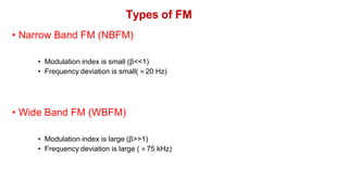
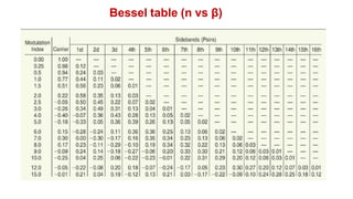
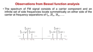
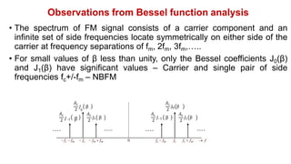
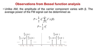
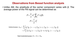
This document discusses two types of frequency modulation (FM): narrowband FM (NBFM) and wideband FM (WBFM). NBFM has a small modulation index and frequency deviation, resulting in an FM signal that is similar to an AM signal but with the lower sideband inverted. WBFM has a large modulation index and frequency deviation, resulting in a non-periodic FM signal that can be represented using its complex envelope and Bessel functions, producing an FM signal with multiple sidebands spaced at integer multiples of the modulating frequency.

1. Types of FM
• Narrow Band FM (NBFM)
• Modulation index is small (β<<1)
• Frequency deviation is small( ≈ 20 Hz)
• Wide Band FM (WBFM)
• Modulation index is large (β>>1)
• Frequency deviation is large ( ≈ 75 kHz)

2. Narrow Band FM
• The FM signal is defined as
s(t)  Ac cos[2fct   sin 2fmt]     (1)
• Expanding Eq.(1), we get (cos(a+b)=cosacosb-sinasinb)

3. Narrow Band FM
• The FM signal is defined as
s(t)  Ac cos[2fct   sin 2fmt]     (1)
• Expanding Eq.(1), we get
s(t)  Accos2fct cos[ sin 2fmt] Acsin 2fctsin[ sin 2fmt]   (2)
• As modulation index β is small, we may use the following
approximations:

4. Narrow Band FM
• The FM signal is defined as
s(t)  Ac cos[2fct   sin 2fmt]     (1)
• Expanding Eq.(1), we get
s(t)  Accos2fct cos[ sin 2fmt] Ac sin 2fctsin[ sin 2fmt]   (2)
• As modulation index β is small, we may use the following
approximations:
• Now Eq.(2) becomes
cos[ sin 2f t] 1
m
sin[ sin 2fmt]   sin 2fmt

5. Narrow Band FM
• The FM signal is defined as
s(t)  Ac cos[2fct   sin 2fmt]     (1)
• Expanding Eq.(1), we get
s(t)  Accos2fct cos[ sin 2fmt] Ac sin 2fctsin[ sin 2fmt]   (2)
• As modulation index β is small, we may use the following
approximations: cos[ sin 2f t] 1
m
sin[ sin 2fmt]   sin 2fmt
• Now Eq.(2) becomes
s(t)  Ac cos2fct  Ac sin 2fctsin 2fmt    (3)
• Eq.(3) defines the approximate form of NBFM signal produced by
sinusoidal message signal

6. Narrow Band FM
• Expanding Eq.(3), we get
2
m
c
c c m
c c
s(t)  A cos2f t 
1
A {cos[2( f  f )t ] cos[2( f  f )t]}  (4)

7. Narrow Band FM
• Expanding Eq.(3), we get
• The above equation is somewhat similar to AM signal
2
m
c
c c m
c c
s(t)  A cos2f t 
1
A {cos[2( f  f )t]  cos[2( f  f )t]}  (4)
2
m
c
c c m
c c
s(t)  A cos2f t 
1
mA {cos[2( f  f )t ] cos[2( f  f )t]}  (5)

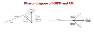
8. Narrow Band FM
• Expanding Eq.(3), we get
• The above equation is somewhat similar to AM signal
• The difference between the two signals is the algebric sign of the lower
side frequency in the narrow band FM is reversed
• The NBFM signal requires the same transmission bandwidth of the AM
signal (2fm)
2
m
c
c c m
c c
s(t)  A cos2f t 
1
A {cos[2( f  f )t]  cos[2( f  f )t]}  (4)
2
m
c
c c m
c c
s(t)  A cos2f t 
1
mA {cos[2( f  f )t]  cos[2( f  f )t]}  (5)

9. Phasor diagram of NBFM and AM

10. Phasor diagram of NBFM and AM
• In NBFM, the resultant phasor has same amplitude of the carrier
phasor but out of phase w.r.t it
• In AM, the resultant phasor has different amplitude of the carrier phasor
but always inphase w.r.t it

11. Narrow Band FM
• Ideally FM signal contains constant envelope
• But here the FM signal produced differs from ideal condition
• The envelope contains a residual amplitude modulation and varies in time
• For a sinusoidal message signal, the angle θi(t) contains harmonic distortion in
the form of third and higher harmonics of fm
• By restricting   0.3 , the effect of residual AM and harmonic distortion
can be limited to negligible levels

12. Wide Band FM
• The FM signal is defined as
s(t)  Ac cos[2fct   sin 2fmt]     (1)
• Eq.(1) is non-periodic unless the carrier signal frequency fc
integral multiple of the message signal frequency fm
• Assume the carrier signal frequency fc is large
is an
• Rewriting Eq.(1) by using complex representation of band-pass signals,
we get

13. Wide Band FM
• The FM signal is defined as
s(t)  Ac cos[2fct   sin 2fmt]     (1)
• Eq.(1) is non-periodic unless the carrier signal frequency fc
integral multiple of the message signal frequency fm
• Assume the carrier signal frequency fc is large
is an
• Rewriting Eq.(1) by using complex representation of band-pass signals,
we get
m
c
c
s(t)  Re[A exp( j2f t  j sin 2f t)]

14. Wide Band FM
• The FM signal is defined as
s(t)  Ac cos[2fct   sin 2fmt]     (1)
• Eq.(1) is non-periodic unless the carrier signal frequency fc
integral multiple of the message signal frequency fm
• Assume the carrier signal frequency fc is large
is an
• Rewriting Eq.(1) by using complex representation of band-pass signals,
we get
c c m
s(t)  Re[A exp( j2f t  j sin 2f t)]
c
s(t)  Re[~
s (t)exp( j2f t)]   (2)
• where ~
s(t)is the complex envelope of the FM signal defined as

15. Wide Band FM
• The FM signal is defined as
s(t)  Ac cos[2fct   sin 2fmt]     (1)
• Eq.(1) is non-periodic unless the carrier signal frequency fc
integral multiple of the message signal frequency fm
• Assume the carrier signal frequency fc is large
is an
• Rewriting Eq.(1) by using complex representation of band-pass signals,
we get
c c m
s(t)  Re[A exp( j2f t  j sin 2f t)]
c
s(t)  Re[~
s (t)exp( j2f t)]   (2)
• where ~
s(t)is the complex envelope of the FM signal defined as
~
s (t)  A exp[ j sin 2f t]   (3)
c m
• ~
s (t) is a periodic function of time with fundamental frequency fm

16. Wide Band FM

17. Wide Band FM
~
s (t)  A exp[ j sin 2f t]   (3)
c m
• Expand ~
s(t) in the form of complex Fourier series is given as
• Cn – Complex Fourier coefficient

~
s(t)  
n
cn exp[ j2nfmt]   (4)

18. Wide Band FM
~
s (t)  A exp[ j sin 2f t]   (3)
c m
• Expand ~
s(t) in the form of complex Fourier series is given as
• Cn – Complex Fourier coefficient
• Sub Eq.(3) in Eq.(5)

~
s(t)  
n
cn exp[ j2nfmt]   (4)
1
1
c  f 
2 fm

2 fm
m
~
s (t)exp( j2nf t)dt    (5)
m
n

19. Wide Band FM
~
s (t)  A exp[ j sin 2f t]   (3)
c m
• Expand ~
s(t) in the form of complex Fourier series is given as
• Cn – Complex Fourier coefficient
• Sub Eq.(3) in Eq.(5)
1

~
s(t)  
n
cn exp[ j2nfmt]   (4)
2 fm
cn  Ac fm exp( j sin 2fmt  j2nfmt)dt    (6)
1

2 fm
1
1
c  f 
2 fm

2 fm
m
~
s (t)exp( j2nf t)dt    (5)
m
n

20. Wide Band FM
• Define a new variable,
• Now the limits become
x  2fmt,
dx  2fmdt

21. Wide Band FM
• Define a new variable,
• Now the limits become
when t  
• Rewrite Eq.(6),
x  2fmt,
dx  2fmdt
, x  
, x  ,
when t 
2 fm
2 fm
1
1

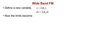
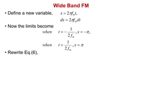
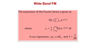
22. Wide Band FM
• Define a new variable,
• Rewrite Eq.(6),
• The integral on the right side of the equation except the scaling factor is
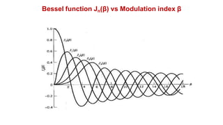
recognized as nth order Bessel function of the 1st kind and argument β.
This function is defined by Jn(β)
x  2fmt,
dx  2fmdt
• Now the limits become
when t  
, x  
, x  ,
when t 
2 fm
2 fm
1
1
exp[ j( sin x  nx)]dx    (7)
c  
Ac
2
n



23. Wide Band FM
1 

• Now Eq.(7) is reduced to
Jn () 
2 exp[ j( sin x  nx)]dx    (8)

24. Wide Band FM
1 
Jn () 
2 exp[ j( sin x  nx)]dx    (8)

• Now Eq.(7) is reduced to
cn  Ac Jn ()    (9)
• Sub Eq.(9) in Eq.(4)

25. Wide Band FM
• Sub Eq.(10) in Eq.(2)
1 
Jn () 
2 exp[ j( sin x  nx)]dx    (8)

• Now Eq.(7) is reduced to
cn  Ac Jn ()    (9)
• Sub Eq.(9) in Eq.(4) 
n
~
s (t)  A J ()exp[ j2nf t]   (10)
c
 n m

26. Wide Band FM
• Sub Eq.(10) in Eq.(2)
• Interchanging the order of the summation and evaluation of the real
part in the R.H.S,
1 
Jn () 
2 exp[ j( sin x  nx)]dx    (8)

• Now Eq.(7) is reduced to
cn  Ac Jn ()    (9)
• Sub Eq.(9) in Eq.(4) 
n
~
s (t)  A J ()exp[ j2nf t]   (10)
c
 n m

s(t)  Ac.Re[ Jn ()exp[ j2( fc  nfm )t]   (11)
n

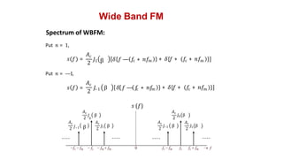
27. Wide Band FM
• By taking Fourier transform, Eq.(12) becomes

s(t)  Ac Jn ()cos[2( fc  nfm )t]   (12)
n
• Eq.(12) is the Fourier series representation of the single tone FM signal
for an arbitrary value of β

28. Wide Band FM
• By taking Fourier transform, Eq.(12) becomes

s(t)  Ac Jn ()cos[2( fc  nfm )t]   (12)
n
• Eq.(12) is the Fourier series representation of the single tone FM signal
for an arbitrary value of β
2
S( f ) 
Ac
m
c


n
Jn ()[( f  fc  nfm ) ( f  f  nf )]   (13)
Put 𝑛 = 0,
⟹ 𝑠 𝑓 =
𝐴c
2
𝐽0  𝛿 𝑓 —𝑓c + 𝛿 𝑓 + 𝑓c

29. Wide Band FM
Spectrum of WBFM:
Put 𝑛 = 1,
𝐴c
2 c
𝐽1 β 𝛿 𝑓 — 𝑓 + 𝑛𝑓m c
+ 𝛿 𝑓 + 𝑓 + 𝑛𝑓m
𝑠 𝑓 =
Put 𝑛 = —1,
𝑠 𝑓 =
𝐴c
2 –1 c
𝐽 β 𝛿 𝑓 — 𝑓 + 𝑛𝑓
m c
+ 𝛿 𝑓 + 𝑓 + 𝑛𝑓m
fc  fm  fc  fm  fm fc  fm fc fc  fm  f
0
𝐴c
2
𝐽 β
0
𝐴c
2
𝐽 β
1
𝐴c
2
𝐽 β
–1
𝐴c
2
𝐽 β
0
𝐴c
2
𝐽 β
1
𝐴c
2 𝐽–1 β
𝑠 (𝑓)

30. Bessel function Jn(β) vs Modulation index β

31. Properties of Bessel function Jn(β)
1. Jn ()  (1) J ()
n n
for all values of n both positive and negative
2. For small values of β
J0 () 1
3.
2
1
Jn ()  0,n  2
J () 


J 2
n () 1
n

33. Bessel table (n vs β)

34. Observations from Bessel function analysis
• The spectrum of FM signal consists of a carrier component and an
infinite set of side frequencies locate symmetrically on either side of the
carrier at frequency separations of fm, 2fm, 3fm,…..
fc  fm  fc  fm  fm fc  fm fc fc  fm  f
0
𝐴c
2
𝐽 β
0
𝐴c
2
𝐽 β
1
𝐴c
2
𝐽 β
–1
𝐴c
2
𝐽 β
0
𝐴c
2
𝐽 β
1
𝐴c
2 𝐽–1 β

35. Observations from Bessel function analysis
• The spectrum of FM signal consists of a carrier component and an
infinite set of side frequencies locate symmetrically on either side of the
carrier at frequency separations of fm, 2fm, 3fm,…..
• For small values of β less than unity, only the Bessel coefficients J0(β)
and J1(β) have significant values – Carrier and single pair of side
frequencies fc+/-fm – NBFM
fc  fm  fc  fm  fm fc  fm fc fc  fm  f
0
𝐴c
2
𝐽 β
0
𝐴c
2
𝐽 β
1
𝐴c
2
𝐽 β
–1
𝐴c
2
𝐽 β
0
𝐴c
2
𝐽 β
1
𝐴c
2 𝐽–1 β

36. Observations from Bessel function analysis
• Unlike AM, the amplitude of the carrier component varies with β. The
average power of the FM signal can be determined as

n
c 
P  J 2
n ()
A
1
2
2
2
1
2
c
A
P 
fc  fm  fc  fm  fm fc  fm fc fc  fm  f
0
𝐴c
2
𝐽 β
0
𝐴c
2
𝐽 β
1
𝐴c
2
𝐽 β
–1
𝐴c
2
𝐽 β
0
𝐴c
2
𝐽 β
1
𝐴c
2 𝐽–1 β

37. Observations from Bessel function analysis
• Unlike AM, the amplitude of the carrier component varies with β. The
average power of the FM signal can be determined as

n
c 
P  J 2
n ()
A
1
2
2
2
1
2
c
A
P 
Sideband power, 𝑃SB =
2
2 2 2 2
𝐽1 β + ⋯ + 𝐽n β + 𝐽–1 β + ⋯ + 𝐽–n β
= 2
𝐴C
2
2
2
𝐽1 β
2
+ ⋯ + 𝐽n β = 𝐴C
2
𝐽1
2
β
2
+ ⋯ + 𝐽n β
𝐴C
2
Total modulated power, 𝑃T = 𝑃C + 𝑃SB