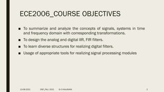
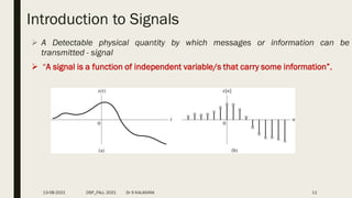
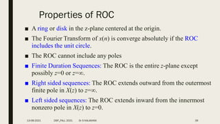
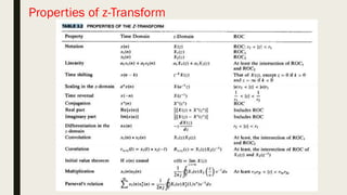
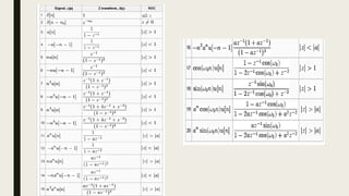
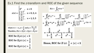
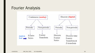
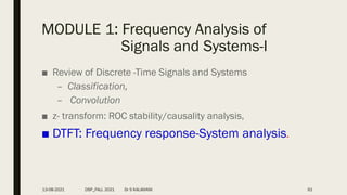
This document outlines the syllabus and course objectives for the digital signal processing course ECE2006 being offered in the fall semester of 2021. The course aims to teach students concepts related to signals and systems in the time and frequency domains, design of analog and digital filters, and realization of digital filters using various structures. The syllabus is divided into 7 modules covering topics such as Fourier analysis, design of IIR and FIR filters, and realization of lattice filters. Students will be evaluated through continuous assessments, quizzes, assignments, and a final exam.

1. ECE2006
DIGITAL SIGNAL PROCESSING
FALL SEMESTER_2021
13-08-2021 DSP_FALL 2021 Dr S KALAIVANI 1

2. ECE2006_COURSE OBJECTIVES
■ To summarize and analyze the concepts of signals, systems in time
and frequency domain with corresponding transformations.
■ To design the analog and digital IIR, FIR filters.
■ To learn diverse structures for realizing digital filters.
■ Usage of appropriate tools for realizing signal processing modules
13-08-2021 DSP_FALL 2021 Dr S KALAIVANI 2

3. Course Outcomes:
1. Comprehend, classify and analyze the signals and systems, also, transform
the time domain signals and response of the system to frequency domain
2. Able to simplify Fourier transform computations using fast algorithms
3. Comprehend the various analog filter design techniques and their digitization.
4. Able to design digital filters.
5. Able to realize digital filters using delay elements, summer, etc
6. Able to realize lattice filters using delay elements, ladders, summers, etc.
7. Able to analyze and exploit the real-time signal processing
application8.Design and implement systems using the imbibed signal
processing concepts
13-08-2021 DSP_FALL 2021 Dr S KALAIVANI 3

4. SYLLABUS
13-08-2021 DSP_FALL 2021 Dr S KALAIVANI 4

5. SYLLABUS
13-08-2021 DSP_FALL 2021 Dr S KALAIVANI 5

6. Mode of Evaluation:
■ Continuous Assessment Test –I (CAT-I) - 15 Marks
■ Continuous Assessment Test –II (CAT-II) -15 Marks
■ Digital Assignments/ Quiz - 30 Marks
– QUIZ_1 - Module 1 and 2
– QUIZ_2 - Module 3 and 4
– DIGITAL ASSIGNMENT - Module 5 and 6
& 7
■ Final Assessment Test (FAT) - 40 Marks
13-08-2021 DSP_FALL 2021 Dr S KALAIVANI 6

7. Introduction
 Need for DSP: To Process real world analog signals -Analog-to-digital conversion
 Signal Processing - Operations on Signals
■ Advantages of DSP:
■ Digital circuits are less sensitive to temperature, ageing & other external parameters.
■ Digital processing is stable, reliable, flexible and repeatable.
■ Easy storage, Accuracy, Less processing cost and maintenance.
■ Covers wide range of frequencies.
■ No loading problems and Multi rate processing is possible
■ Highly suitable for processing low frequency signal also.
■ Disadvantages of DSP:
■ Pre and Post processing devices – Increases the complexity of the system
■ High power consumption
■ Frequency limitations
13-08-2021 DSP_FALL 2021 Dr S KALAIVANI 7

8. 8
Applications of DSP
13-08-2021 DSP_FALL 2021 Dr S KALAIVANI

9. 9
DIGITAL SIGNAL PROCESSING
Module Description
I & II Frequency Analysis of Signals and Systems-I and II
III Theory and Design of Analog Filters
IV Design of Digital IIR Filter
V Design of Digital FIR Filters
VI Realization of Digital Filters
VII Realization of Lattice filter structures
13-08-2021 DSP_FALL 2021 Dr S KALAIVANI

10. MODULE 1: Frequency Analysis of
Signals and Systems-I
■ Review of Discrete -Time Signals and Systems
– Classification,
– Convolution
■ z- transform: ROC stability/causality analysis,
■ DTFT: Frequency response-System analysis.
13-08-2021 DSP_FALL 2021 Dr S KALAIVANI 10

11. Introduction to Signals
 A Detectable physical quantity by which messages or information can be
transmitted - signal
 “A signal is a function of independent variable/s that carry some information”.
13-08-2021 DSP_FALL 2021 Dr S KALAIVANI 11

12. REPRESENTATION OF DT SIGNALS
Graphical Representation
2
)
3
(
,
1
)
2
(
,
3
)
1
(
,
0
)
0
(
,
2
)
1
(
,
3
)
2
( 







 x
x
x
x
x
x
Functional Representation
Sequence Representation
Tabular Representation
13-08-2021 DSP_FALL 2021 Dr S KALAIVANI 12

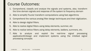
13. 1. Unit Impulse Signal
2. Unit Step Signal
3. Unit Ramp Signal
4. Sinusoidal Signal
5. Exponential Signal
13
BASIC SIGNALS 0
0
0
1
]
[



n
for
n
for
n

0
0
0
1
]
[



n
for
n
for
n
u
0
0
0
]
[



n
for
n
for
n
n
r
)
cos(
]
[ 
 
 n
A
n
x
T
F 

 2
2 



n
a
n
x n

 ;
]
[
13-08-2021 DSP_FALL 2021 Dr S KALAIVANI

14. ■ CT and DT signals are further classified as,
– Deterministic and Random
– Periodic and Non-periodic
– Causal and Non Causal
– Even and Odd
– Energy and Power 14
CLASSIFICATION OF SIGNALS
Basic operations on signals
13-08-2021 DSP_FALL 2021 Dr S KALAIVANI

15. Classification of Signals
■ CT and DT signals are further classified as,
– Deterministic and Random
– Periodic and Non-periodic
– Causal and Non Causal
– Even and Odd
– Energy and Power
13-08-2021 DSP_FALL 2021 Dr S KALAIVANI 15

16. ■ Example :
The signal is given below is energy or power signal.
Explain.
16
Power and Energy
 
x n
 
x n
3
0 1
n
2
13-08-2021 DSP_FALL 2021 Dr S KALAIVANI

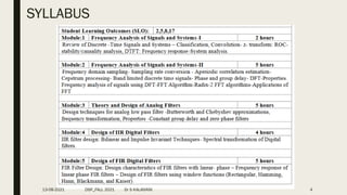
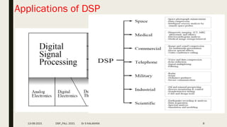
17. • Systems process input signals to produce output signals
– Continuous/Discrete
– Linear/Non linear
– Causal/Non Causal
– Stable/Unstable
– Dynamic/Static
– Time variance/Time invariant
17
Classification of Systems
 Causal: a system is causal if the output at a time, only depends on input values up to that time.
 Linear: a system is linear if the output of the scaled sum of two input signals is the equivalent scaled
sum of outputs
 Time-invariance: a system is time invariant if the system’s output is the same, given the same input
signal, regardless of time.
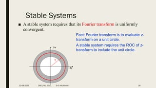
 A system is called stable in the bounded-input bounded-output (BIBO) sense if every bounded input
sequence produces a bounded output sequence
 A system is called memoryless /Static if the output y[n] at every value of n depends only on the
present input values of n
13-08-2021 DSP_FALL 2021 Dr S KALAIVANI

18. Ex. Y[n]=x[-n]
13-08-2021 DSP_FALL 2021 Dr S KALAIVANI 18

19. MODULE 1: Frequency Analysis of
Signals and Systems-I
■ Review of Discrete -Time Signals and Systems
– Classification,
– Convolution
■ z- transform: ROC stability/causality analysis,
■ DTFT: Frequency response-System analysis.
13-08-2021 DSP_FALL 2021 Dr S KALAIVANI 19

20. Convolution
■ The output sequence y(n) is found as,
This is called convolution sum.
DSP_FALL 2021 Dr S KALAIVANI 20
13-08-2021

21. Determine the response of the system for the following input signal
and impulse response.
x(n)={1,2,1}, h(n)={1,2,3}
21
13-08-2021 DSP_FALL 2021 Dr S KALAIVANI

22. Circular Convolution
The circular convolution of two sequences x1(n) and x2(n) is
defined as
However it is not the ordinary linear convolution that was
discussed in previous section, which relates the output sequence
y(n) of a linear system to the input sequence x(n) and the impulse
response h(n). Instead, the convolution sum involves the index
x2((m-n))N and is called circular convolution.
If the two sequences x(n) and h(n) contain L and M number of
samples respectively and that L > M, then to perform circular
convolution between the two using N=Max(L,M), the L – M
number of zero samples to be added to the sequence h(n), so
that both the sequences are periodic with N
1
3 1 2
0
( ) ( ) (( ))
N
N
n
x m x n x m n


 

22
13-08-2021 DSP_FALL 2021 Dr S KALAIVANI

23. Circular Convolution for N=8
23
13-08-2021 DSP_FALL 2021 Dr S KALAIVANI

24. Perform the circular convolution of the following two sequences.
x1(n)={1,2,1}, x2(n)={1,2,3}
24
13-08-2021 DSP_FALL 2021 Dr S KALAIVANI

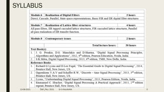
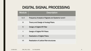
25. Ex.1 Find the linear and circular (7-point) convolution of the
given sequences
x[n]={1, 2, 7, -2, 3, -1, 5} and h[n]={-1, 3, 5, -3, 1}
■ Linear Convolution:
y[n]={-1, 1, 4, 30, 21, -19, 20, -1, 31, -15,5}
■ Circular Convolution:
x[n]={1, 2, 7, -2, 3, -1, 5}
h[n]={-1, 3, 5, -3, 1, 0, 0}
y[n]={-2, 32,-12,35,21,20}
13-08-2021 DSP_FALL 2021 Dr S KALAIVANI 25

26. MODULE 1: Frequency Analysis of
Signals and Systems-I
■ Review of Discrete -Time Signals and Systems
– Classification,
– Convolution
■ z- transform: ROC stability/causality analysis,
■ DTFT: Frequency response-System analysis.
13-08-2021 DSP_FALL 2021 Dr S KALAIVANI 26

27. z-transform
*A generalization of Fourier transform
■ The z-transform of sequence x(n) is defined by






n
n
z
n
x
z
X )
(
)
(
Re
Im
z = ej

■ Give a sequence, the set of values of z for which the z-transform
converges, i.e., |X(z)|<, is called the region of convergence.



 









n
n
n
n
z
n
x
z
n
x
z
X |
||
)
(
|
)
(
|
)
(
|
ROC is centered on origin and consists of a set of rings.
13-08-2021 DSP_FALL 2021 Dr S KALAIVANI 27

28. Stable Systems
■ A stable system requires that its Fourier transform is uniformly
convergent.
Re
Im
1
Fact: Fourier transform is to evaluate z-
transform on a unit circle.
A stable system requires the ROC of z-
transform to include the unit circle.
13-08-2021 DSP_FALL 2021 Dr S KALAIVANI 28

29. Example: A right sided Sequence
)
(
)
( n
u
a
n
x n

n
n
n
z
n
u
a
z
X 




 )
(
)
(





0
n
n
n
z
a





0
1
)
(
n
n
az
For convergence of X(z), we require that






0
1
|
|
n
az 1
|
| 1


az
|
|
|
| a
z 
a
z
z
az
az
z
X
n
n




 



 1
0
1
1
1
)
(
)
(
|
|
|
| a
z 
13-08-2021 DSP_FALL 2021 Dr S KALAIVANI 29

30. a
a
Example: A right sided Sequence ROC
for x(n)=anu(n)
|
|
|
|
,
)
( a
z
a
z
z
z
X 


Re
Im
1
a
a
Re
Im
1
Which one is stable?
13-08-2021 DSP_FALL 2021 Dr S KALAIVANI 30

31. Example: A left sided Sequence
)
1
(
)
( 


 n
u
a
n
x n
n
n
n
z
n
u
a
z
X 



 


 )
1
(
)
(
For convergence of X(z), we require that






0
1
|
|
n
z
a 1
|
| 1


z
a
|
|
|
| a
z 
a
z
z
z
a
z
a
z
X
n
n






 



 1
0
1
1
1
1
)
(
1
)
(
|
|
|
| a
z 
n
n
n
z
a 






1
n
n
n
z
a






1
n
n
n
z
a






0
1
13-08-2021 DSP_FALL 2021 Dr S KALAIVANI 31

32. a
a
Example: A left sided Sequence ROC
for x(n)=anu( n1)
|
|
|
|
,
)
( a
z
a
z
z
z
X 


Re
Im
1
a
a
Re
Im
1
Which one is stable?
13-08-2021 DSP_FALL 2021 Dr S KALAIVANI 32

33. Represent z-transform as a Rational Function
)
(
)
(
)
(
z
Q
z
P
z
X 
where P(z) and Q(z) are
polynomials in z.
Zeros: The values of z’s such that X(z) = 0
Poles: The values of z’s such that X(z) = 
13-08-2021 DSP_FALL 2021 Dr S KALAIVANI 33

34. Example: A right sided Sequence
)
(
)
( n
u
a
n
x n
 |
|
|
|
,
)
( a
z
a
z
z
z
X 


Re
Im
a
ROC is bounded by
the pole and is the
exterior of a circle.
13-08-2021 DSP_FALL 2021 Dr S KALAIVANI 34

35. Example: A left sided Sequence
)
1
(
)
( 


 n
u
a
n
x n
|
|
|
|
,
)
( a
z
a
z
z
z
X 


Re
Im
a
ROC is bounded by
the pole and is the
interior of a circle.
13-08-2021 DSP_FALL 2021 Dr S KALAIVANI 35

36. Example: Sum of Two Right Sided Sequences
)
(
)
(
)
(
)
(
)
( 3
1
2
1
n
u
n
u
n
x n
n



3
1
2
1
)
(




z
z
z
z
z
X
Re
Im
1/2
)
)(
(
)
(
2
3
1
2
1
12
1




z
z
z
z
1/3
1/12
ROC is bounded by poles
and is the exterior of a
circle.
ROC does not include any pole.
13-08-2021 DSP_FALL 2021 Dr S KALAIVANI 36

37. Example: A Two Sided Sequence
)
1
(
)
(
)
(
)
(
)
( 2
1
3
1




 n
u
n
u
n
x n
n
2
1
3
1
)
(




z
z
z
z
z
X
Re
Im
1/2
)
)(
(
)
(
2
2
1
3
1
12
1




z
z
z
z
1/3
1/12
ROC is bounded by poles
and is a ring.
ROC does not include any pole.
13-08-2021 DSP_FALL 2021 Dr S KALAIVANI 37

38. Example: A Finite Sequence
1
0
,
)
( 


 N
n
a
n
x n
n
N
n
n
N
n
n
z
a
z
a
z
X )
(
)
( 1
1
0
1
0







 

Re
Im
ROC: 0 < z < 
ROC does not include any pole.
1
1
1
)
(
1





az
az N
a
z
a
z
z
N
N
N


 1
1
N-1 poles
N-1 zeros
Always Stable
13-08-2021 DSP_FALL 2021 Dr S KALAIVANI 38

39. Properties of ROC
■ A ring or disk in the z-plane centered at the origin.
■ The Fourier Transform of x(n) is converge absolutely if the ROC
includes the unit circle.
■ The ROC cannot include any poles
■ Finite Duration Sequences: The ROC is the entire z-plane except
possibly z=0 or z=.
■ Right sided sequences: The ROC extends outward from the outermost
finite pole in X(z) to z=.
■ Left sided sequences: The ROC extends inward from the innermost
nonzero pole in X(z) to z=0.
13-08-2021 DSP_FALL 2021 Dr S KALAIVANI 39

40. Properties of z-Transform

42. Ex.1 Find the z-transform and ROC of the given sequence

43. INVERSE Z-TRANSFORM
Partial Fraction Method
13-08-2021 DSP_FALL 2021 Dr S KALAIVANI 43

44. Example: 2nd Order Z-Transform
44
 
2
1
z
:
ROC
z
2
1
1
z
4
1
1
1
z
X
1
1


















 

















 1
2
1
1
z
2
1
1
A
z
4
1
1
A
z
X
  1
4
1
2
1
1
1
z
X
z
4
1
1
A 1
4
1
z
1
1 
























 


  2
2
1
4
1
1
1
z
X
z
2
1
1
A 1
2
1
z
1
2 























 


13-08-2021 DSP_FALL 2021 Dr S KALAIVANI

45. Example Continued
■ ROC extends to infinity
– Indicates right sided sequence
45
 
2
1
z
z
2
1
1
2
z
4
1
1
1
z
X
1
1




















     
n
u
4
1
-
n
u
2
1
2
n
x
n
n













a
z
az
n
u
an
|
|
|
,
1
1
)
( 1


 
13-08-2021 DSP_FALL 2021 Dr S KALAIVANI

46. Example #2
*Long division to obtain Bo
46
   
 
1
z
z
1
z
2
1
1
z
1
z
2
1
z
2
3
1
z
z
2
1
z
X
1
1
2
1
2
1
2
1























1
z
5
2
z
3
z
2
1
z
2
z
1
z
2
3
z
2
1
1
1
2
1
2
1
2














 
 
1
1
1
z
1
z
2
1
1
z
5
1
2
z
X















  1
2
1
1
z
1
A
z
2
1
1
A
2
z
X 
 




  9
z
X
z
2
1
1
A
2
1
z
1
1 











    8
z
X
z
1
A
1
z
1
2 




13-08-2021 DSP_FALL 2021 Dr S KALAIVANI

47. Example #2 Continued
*ROC extends to infinity
Indicates right-sides sequence
47
  1
z
z
1
8
z
2
1
1
9
2
z
X 1
1





 

       
n
8u
2
1
9
2 







 n
u
n
n
x
n

  1
2
1
1
z
1
A
z
2
1
1
A
2
z
X 
 




13-08-2021 DSP_FALL 2021 Dr S KALAIVANI

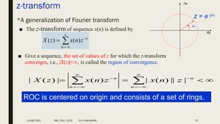
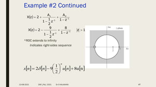
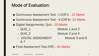
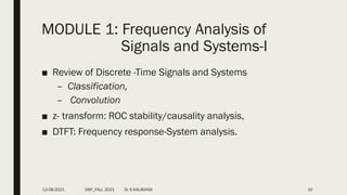
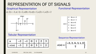
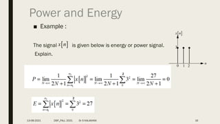
48. Example 3: Find the signal corresponding to the z-transform
48
2
1
3
z
z
3
2
z
)
z
(
X 





Solution:   
5
.
0
z
1
z
z
5
.
0
z
5
.
0
z
5
.
1
z
5
.
0
z
z
3
2
z
)
z
(
X 2
3
2
1
3








 


   5
.
0
z
4
1
z
1
z
1
z
3
5
.
0
z
1
z
z
5
.
0
z
)
z
(
X
2
2










5
.
0
z
z
)
4
(
1
z
z
z
1
3
)
z
(
X







or 1
1
1
z
5
.
0
1
1
4
z
1
1
z
3
)
z
(
X 








  ]
n
[
u
5
.
0
4
]
n
[
u
]
1
n
[
]
n
[
3
]
n
[
x
n








13-08-2021 DSP_FALL 2021 Dr S KALAIVANI

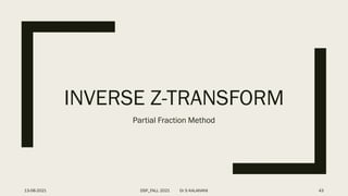
49. Partial Fraction Method:
Example 4: Find the signal corresponding to the z-transform
49
  2
1
1
z
2
.
0
1
z
2
.
0
1
1
)
z
(
Y





Solution:
  2
3
2
.
0
z
2
.
0
z
z
)
z
(
Y



    2
2
2
2
.
0
z
1
.
0
2
.
0
z
75
.
0
2
.
0
z
25
.
0
2
.
0
z
2
.
0
z
z
z
)
z
(
Y









 2
2
.
0
z
z
1
.
0
2
.
0
z
z
75
.
0
1
z
z
25
.
0
)
z
(
Y






 2
1
1
2
.
0
1
.
0
1
1
z
2
.
0
1
z
2
.
0
z
2
.
0
1
1
75
.
0
z
2
.
0
1
1
25
.
0










      ]
n
[
u
2
.
0
n
5
.
0
]
n
[
u
2
.
0
75
.
0
]
n
[
u
2
.
0
25
.
0
]
n
[
y
n
n
n





13-08-2021 DSP_FALL 2021 Dr S KALAIVANI

50. INVERSE Z-TRANSFORM
Power Series Expansion Method
13-08-2021 DSP_FALL 2021 Dr S KALAIVANI 50

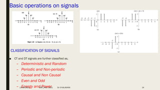
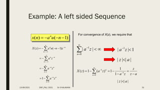
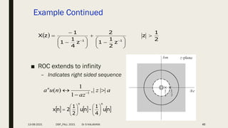
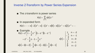
51. Inverse Z-Transform by Power Series Expansion
■ The z-transform is power series
■ In expanded form
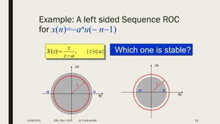
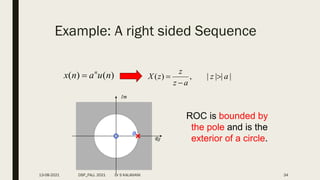
■ Causal/Right sided sequence:
■ Non-Causal/Left sided sequence:
51
   






n
n
z
n
x
z
X
            
 







 
 2
1
1
2
z
2
x
z
1
x
0
x
z
1
x
z
2
x
z
X
        



 
 2
1
2
1
0 z
x
z
x
x
z
X
      1
2
1
2 z
x
z
x
z
X 



 




x[n] ->co-eff of NEGATIVE powers of ‘z’
x[n] ->co-eff of POSITIVE powers of ‘z’
13-08-2021 DSP_FALL 2021 Dr S KALAIVANI

52. Inverse Z-Transform by Power Series Expansion
■ The z-transform is power series
■ In expanded form
■ Example
52
   






n
n
z
n
x
z
X
            
 







 
 2
1
1
2
z
2
x
z
1
x
0
x
z
1
x
z
2
x
z
X
    
1
2
1
1
1
2
z
2
1
1
z
2
1
z
z
1
z
1
z
2
1
1
z
z
X


















         
1
n
2
1
n
1
n
2
1
2
n
n
x 










 



















2
n
0
1
n
2
1
0
n
1
1
n
2
1
2
n
1
n
x
13-08-2021 DSP_FALL 2021 Dr S KALAIVANI

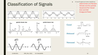
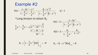
53. Power Series Method
Example 1: Determine the z-transform of RSS
53
2
1
z
5
.
0
z
5
.
1
1
1
)
z
(
X 




By dividing the numerator of X(z) by its
denominator, we obtain the power series
...
z
z
z
z
1
z
z
1
1 4
16
31
3
8
15
2
4
7
1
2
3
2
2
1
1
2
3














 x[n] = [1, 3/2, 7/2, 15/8, 31/16,…. ]
13-08-2021 DSP_FALL 2021 Dr S KALAIVANI

54. Power Series Method
Example 2:Determine the z-transform of
54
2
1
1
z
z
2
2
z
4
)
z
(
X 






By dividing the numerator of X(z) by its
denominator, we obtain the power series
 x[n] = [2, 1.5, 0.5, 0.25, …..]
13-08-2021 DSP_FALL 2021 Dr S KALAIVANI

55. MODULE 1: Frequency Analysis of
Signals and Systems-I
■ Review of Discrete -Time Signals and Systems
– Classification,
– Convolution
■ z- transform: ROC stability/causality analysis,
■ DTFT: Frequency response-System analysis.
13-08-2021 DSP_FALL 2021 Dr S KALAIVANI 55

56. Fourier Analysis
56
13-08-2021 DSP_FALL 2021 Dr S KALAIVANI

57. ■ We have seen that periodic signals can be represented
with the Fourier series
■ Can aperiodic signals be analyzed in terms of frequency
components?
■ Yes, and the Fourier transform provides the tool for this
analysis
■ The major difference w.r.t. the line spectra of periodic
signals is that the spectra of aperiodic signals are defined
for all real values of the frequency variable not just for a
discrete set of values
Fourier Transform

13-08-2021 DSP_FALL 2021 Dr S KALAIVANI 57

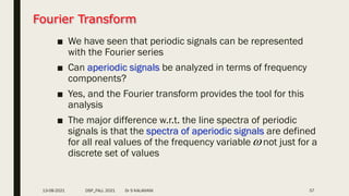
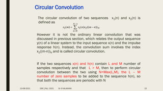
58. The Discrete-Time Fourier Transform
■ The discrete-time Fourier transform (DTFT) or, simply, the Fourier
transform of a discrete–time sequence x[n] is a representation of
the sequence in terms of the complex exponential sequence
where is the real frequency variable.
■ The discrete-time Fourier transform of a sequence x[n] is
defined by
 
j x
e 


 
j
X e 
  [ ]
j j n
n
X e x n e
 



 
 
j x
e 

 
j
X e 
DSP_FALL 2021 Dr S KALAIVANI Discrete-Time Signals in the Transform-Domain 58

59. The Discrete-Time Fourier Transform
■ Convergence Condition:
If x[n] is an absolutely summable sequence, i.e.,
Thus the equation is a sufficient condition for the existence of
the DTFT.
 
     
n
j j n
n n
if x n
then X e x n e x n
 


 

 
 
   

 
13-08-2021 DSP_FALL 2021 Dr S KALAIVANI 59

60. 13-08-2021 DSP_FALL 2021 Dr S KALAIVANI 60

61. MODULE 1: Frequency Analysis of
Signals and Systems-I
■ Review of Discrete -Time Signals and Systems
– Classification,
– Convolution
■ z- transform: ROC stability/causality analysis,
■ DTFT: Frequency response-System analysis.
61
13-08-2021 DSP_FALL 2021 Dr S KALAIVANI

62. DTFT in System Analysis
13-08-2021 DSP_FALL 2021 Dr S KALAIVANI 62

63. 13-08-2021 DSP_FALL 2021 Dr S KALAIVANI 63
DTFT in System Analysis

64. Contd.,
13-08-2021 DSP_FALL 2021 Dr S KALAIVANI 64

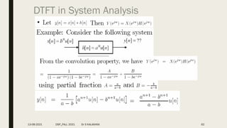
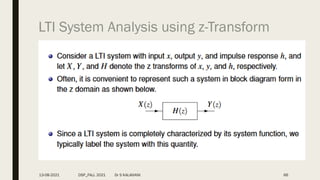
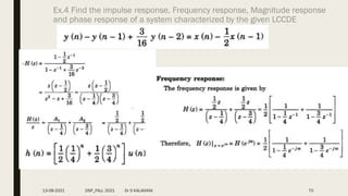
65. Ex. A discrete-time LTI system has impulse response h[n],Find
the output y[n] due to input x[n].
13-08-2021 DSP_FALL 2021 Dr S KALAIVANI 65

66. LTI System Analysis using z-Transform
13-08-2021 DSP_FALL 2021 Dr S KALAIVANI 66

67. Interconnection of LTI system
13-08-2021 DSP_FALL 2021 Dr S KALAIVANI 67

68. Ex.2
13-08-2021 DSP_FALL 2021 Dr S KALAIVANI 68

69. Ex.3
13-08-2021 DSP_FALL 2021 Dr S KALAIVANI 69

70. Ex.4 Find the impulse response, Frequency response, Magnitude response
and phase response of a system characterized by the given LCCDE
13-08-2021 DSP_FALL 2021 Dr S KALAIVANI 70

71. Contd.,
13-08-2021 DSP_FALL 2021 Dr S KALAIVANI 71

72. Ex.4
13-08-2021 DSP_FALL 2021 Dr S KALAIVANI 72

73. Ex.5
13-08-2021 DSP_FALL 2021 Dr S KALAIVANI 73