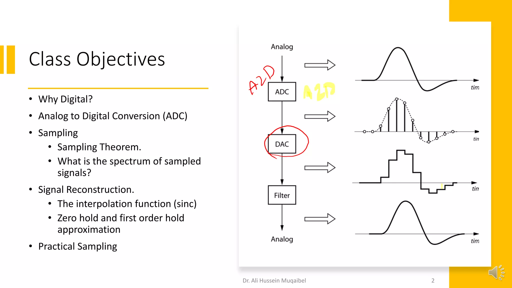
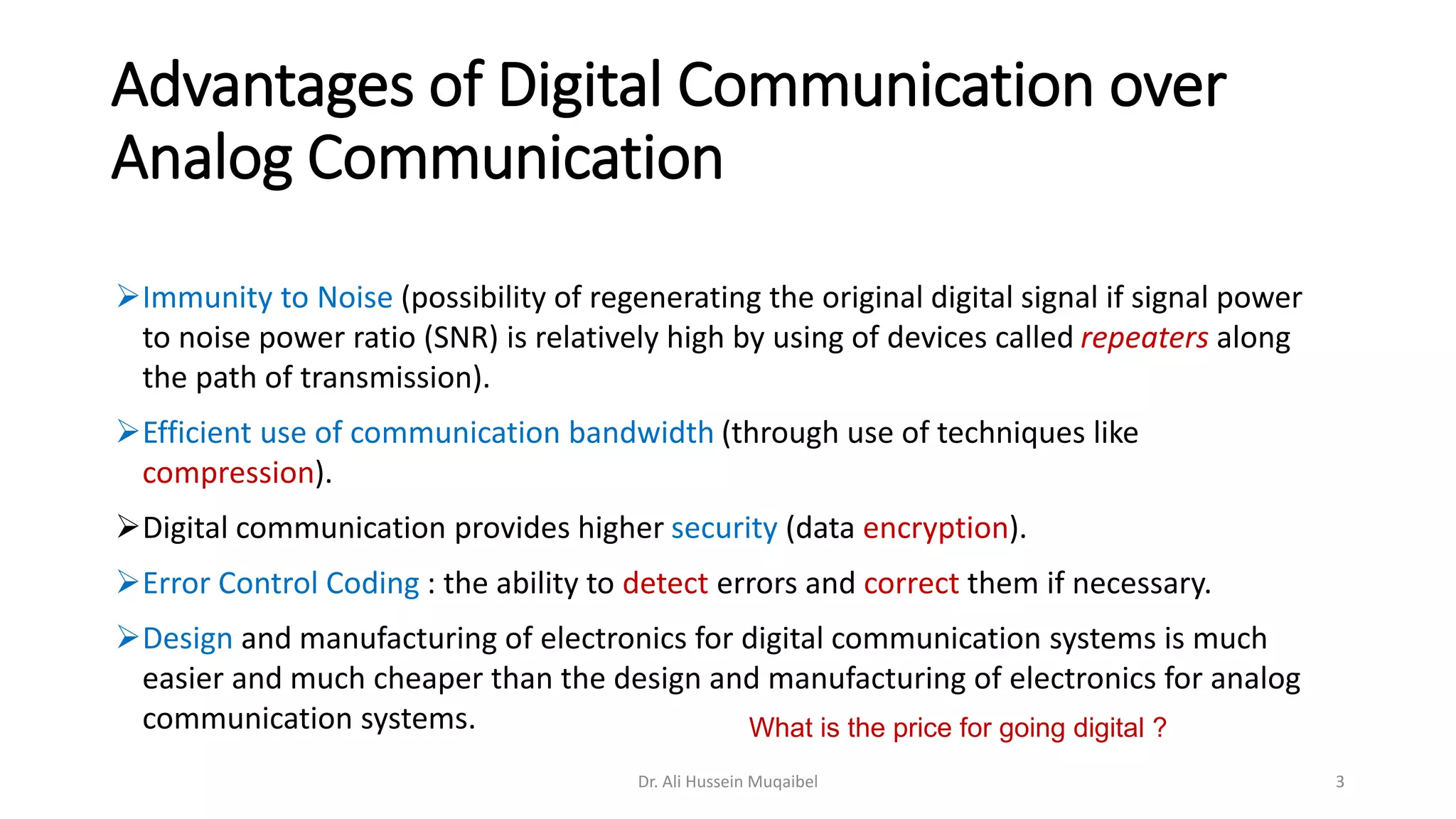
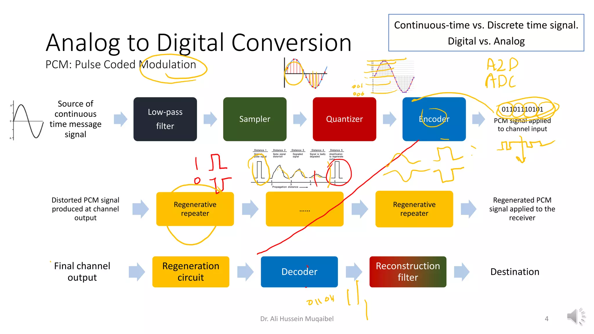
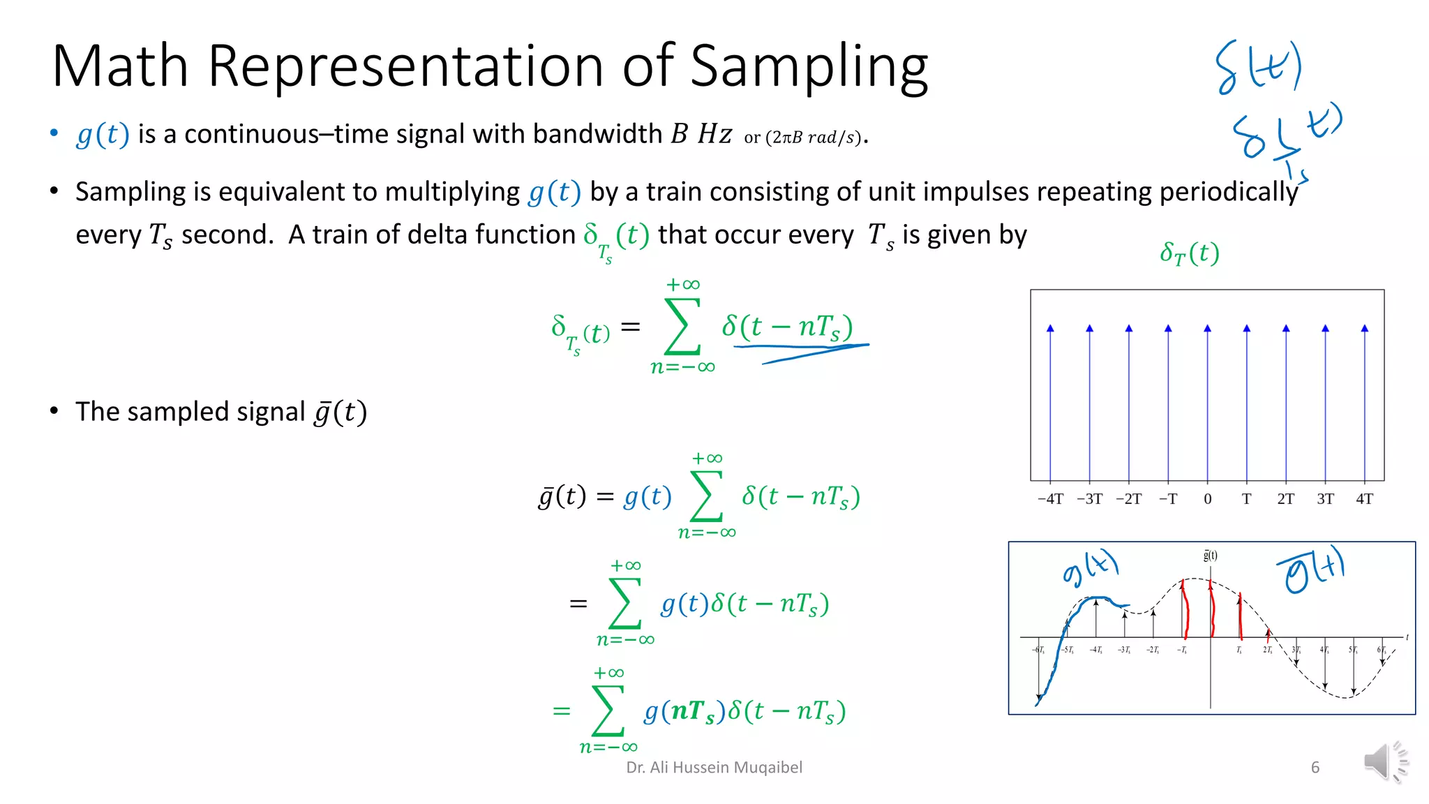
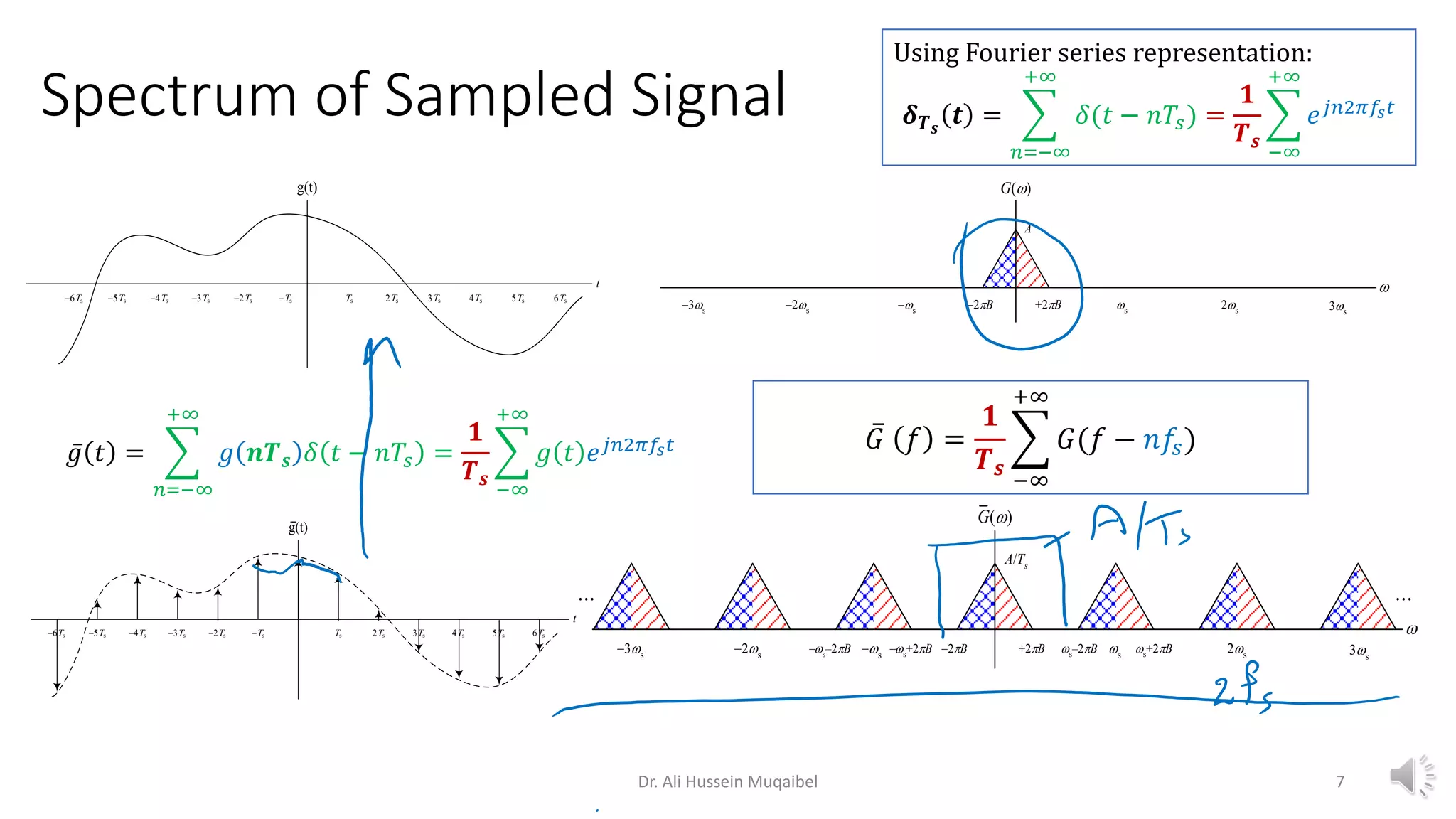
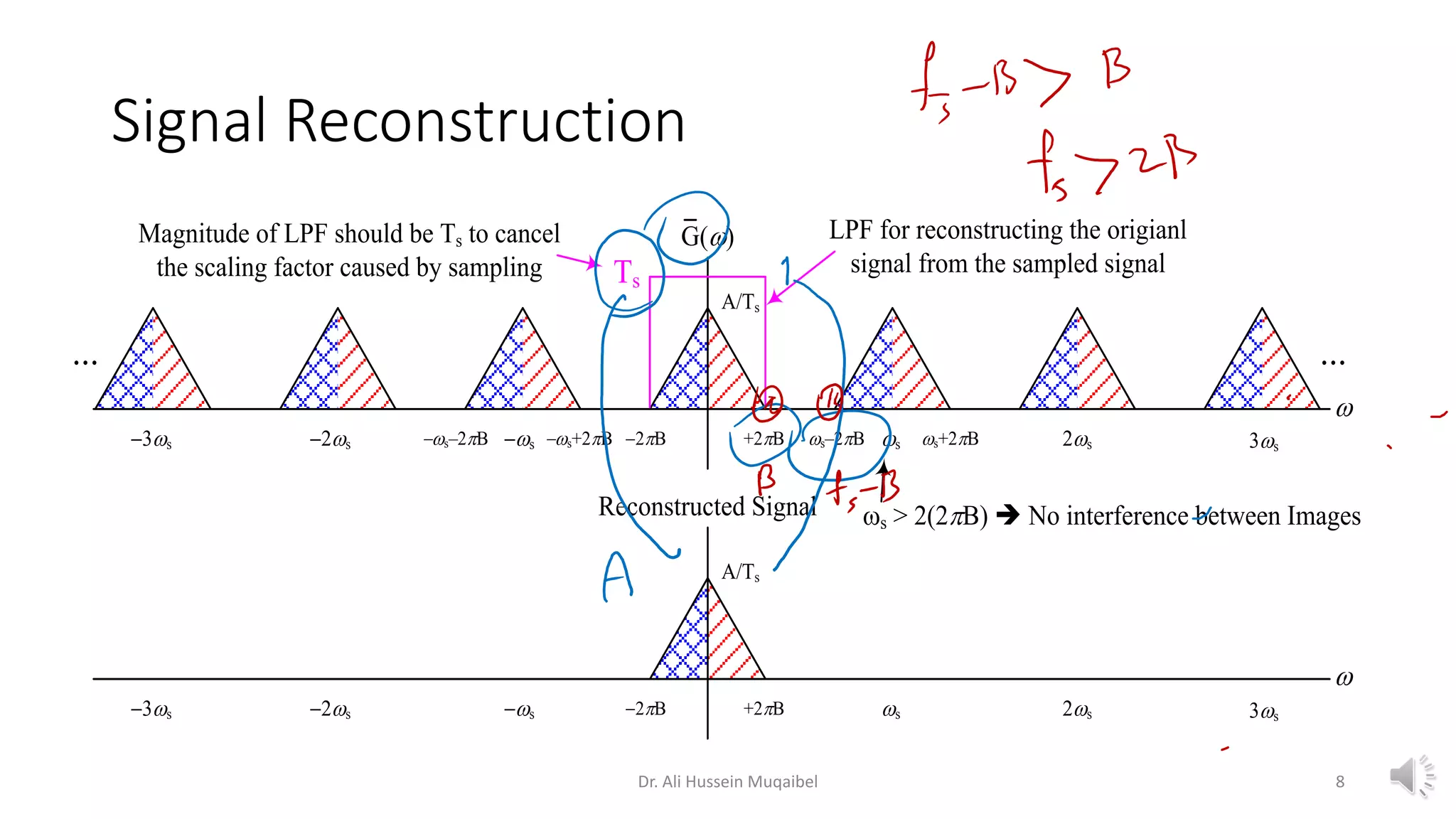
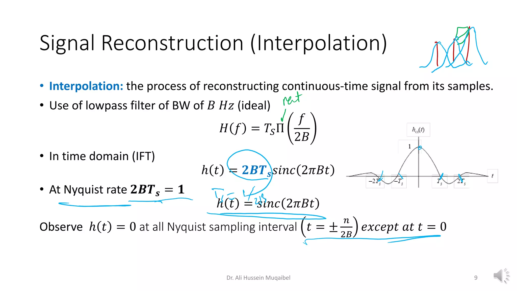
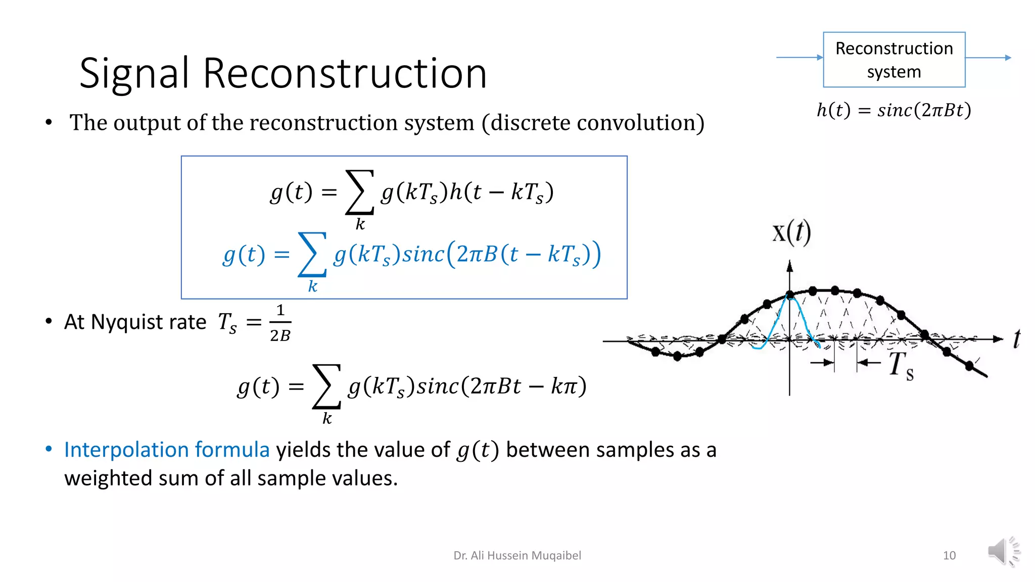
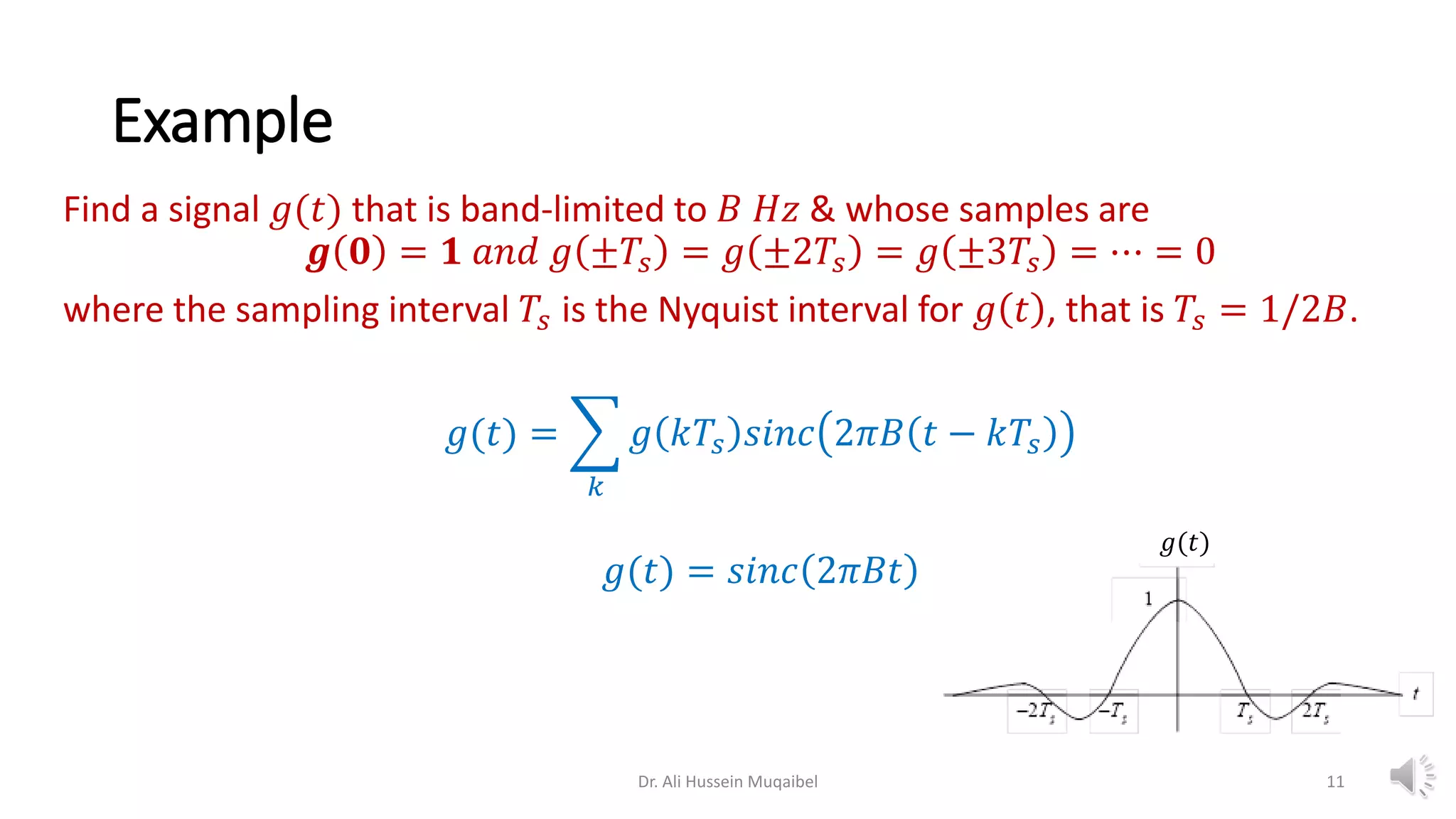
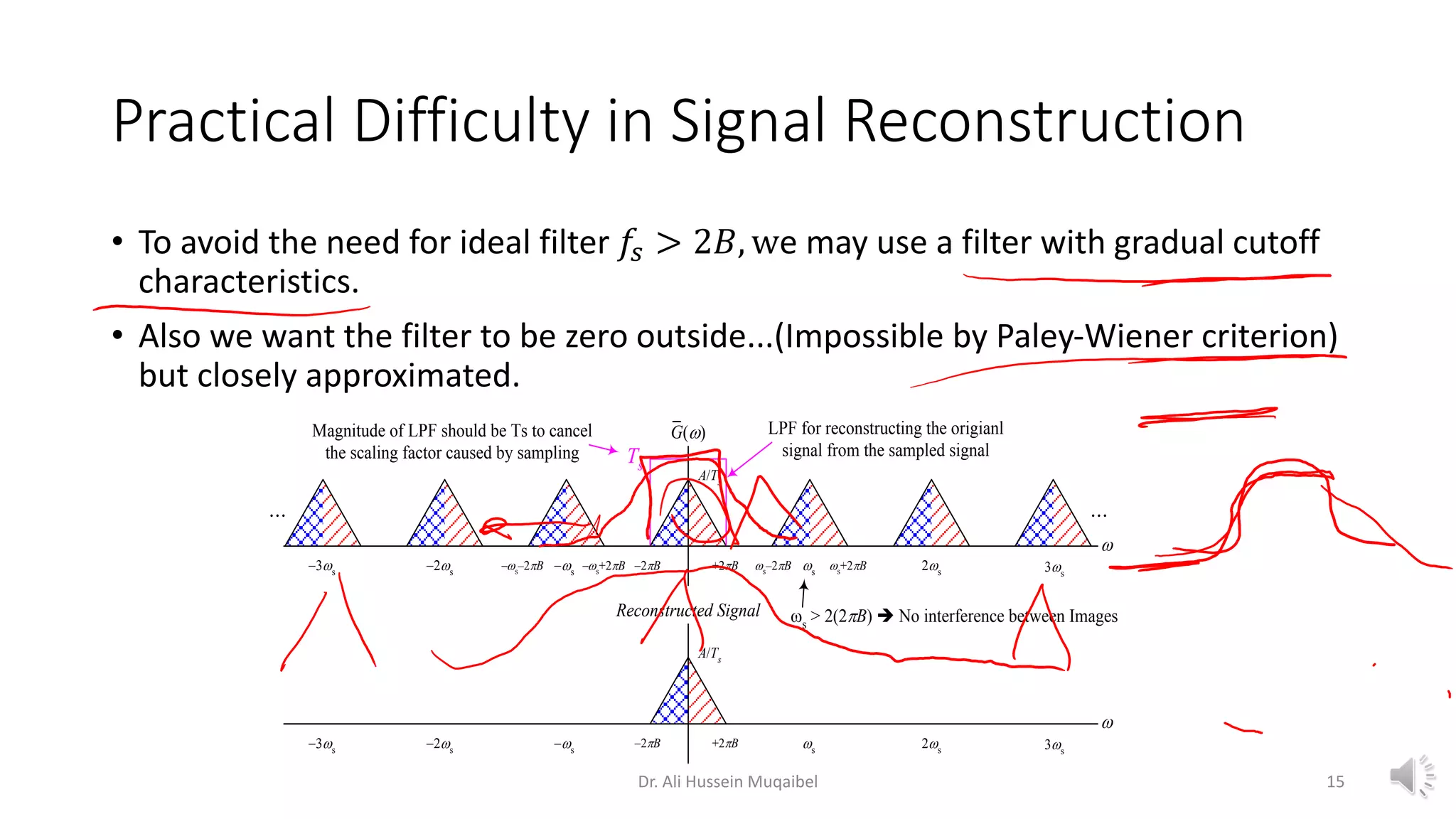
This document discusses analog to digital conversion and signal sampling and reconstruction. It begins by explaining the advantages of digital over analog communication and the process of analog to digital conversion using pulse code modulation. It then covers the sampling theorem, which states that a bandlimited signal can be reconstructed from samples taken at or above the Nyquist rate. The document provides the mathematical representations of sampling and discusses how the spectrum of a sampled signal consists of copies of the original spectrum spaced at integer multiples of the sampling frequency. It describes how reconstruction involves the use of an interpolation filter, such as the sinc function, to filter out copies and reconstruct the original signal from its samples. Finally, it discusses practical considerations in sampling and reconstruction.

1. Sampling
&
Signal Reconstruction
with Applications
Dr. Ali Hussein Muqaibel
ver. 4.5
1
Analog to Digital
Conversion (ADC)
Part I
Digital Transmission
Part II
Digital Communications

2. Class Objectives
• Why Digital?
• Analog to Digital Conversion (ADC)
• Sampling
• Sampling Theorem.
• What is the spectrum of sampled
signals?
• Signal Reconstruction.
• The interpolation function (sinc)
• Zero hold and first order hold
approximation
• Practical Sampling
Dr. Ali Hussein Muqaibel 2

3. Advantages of Digital Communication over
Analog Communication
➢Immunity to Noise (possibility of regenerating the original digital signal if signal power
to noise power ratio (SNR) is relatively high by using of devices called repeaters along
the path of transmission).
➢Efficient use of communication bandwidth (through use of techniques like
compression).
➢Digital communication provides higher security (data encryption).
➢Error Control Coding : the ability to detect errors and correct them if necessary.
➢Design and manufacturing of electronics for digital communication systems is much
easier and much cheaper than the design and manufacturing of electronics for analog
communication systems.
Dr. Ali Hussein Muqaibel 3
What is the price for going digital ?

4. Analog to Digital Conversion
PCM: Pulse Coded Modulation
Source of
continuous
time message
signal
Low-pass
filter
Sampler Quantizer Encoder
01101110101
PCM signal applied
to channel input
Dr. Ali Hussein Muqaibel
Continuous-time vs. Discrete time signal.
Digital vs. Analog
4
Distorted PCM signal
produced at channel
output
Regenerative
repeater
……
Regenerative
repeater
Regenerated PCM
signal applied to the
receiver
Final channel
output
Regeneration
circuit
Decoder
Reconstruction
filter
Destination

5. Sampling Theorem
A signal whose spectrum is band limited to 𝐵 𝐻𝑧
[𝐺(𝑓) = 0 𝑓𝑜𝑟 |𝑓| > 𝐵] can be reconstructed exactly from its samples taken
uniformly at a rate 𝑅 > 2𝐵 𝐻𝑧 (samples/ sec). i.e 𝑇𝑆 <
1
2𝐵
Minimum sampling frequency is 𝑓𝑠 = 2𝐵 𝐻𝑧 𝑁𝑦𝑞𝑢𝑖𝑠𝑡 𝑅𝑎𝑡𝑒
𝑇𝑠 =
1
2𝐵
Nyquist interval
The 𝑛𝑡ℎ impulse located at 𝑡 = 𝑛𝑇𝑠 has a strength 𝑔 𝑛𝑇𝑠 the value of 𝑔(𝑡) at 𝑡 = 𝑛𝑇𝑠
t
s s s s s s
s s s s s s
g(t)
Dr. Ali Hussein Muqaibel
𝑇𝑠 = 1/𝑓𝑠 sampling interval
5

6. Math Representation of Sampling
• 𝑔(𝑡) is a continuous–time signal with bandwidth 𝐵 𝐻𝑧 or (2𝐵 𝑟𝑎𝑑/𝑠).
• Sampling is equivalent to multiplying 𝑔(𝑡) by a train consisting of unit impulses repeating periodically
every 𝑇𝑠 second. A train of delta function 𝑇
𝑠
(𝑡) that occur every 𝑇𝑠 is given by
𝑇
𝑠
𝑡 = ෍
𝑛=−∞
+∞
𝛿(𝑡 − 𝑛𝑇𝑠)
• The sampled signal ҧ
𝑔(𝑡)
ҧ
𝑔 𝑡 = 𝑔(𝑡) ෍
𝑛=−∞
+∞
𝛿(𝑡 − 𝑛𝑇𝑠)
= ෍
𝑛=−∞
+∞
𝑔(𝑡)𝛿(𝑡 − 𝑛𝑇𝑠)
= ෍
𝑛=−∞
+∞
𝑔(𝒏𝑻𝒔)𝛿(𝑡 − 𝑛𝑇𝑠)
Dr. Ali Hussein Muqaibel 6
𝛿𝑇(𝑡)
t
s s s s s s
s s s s s s
g(t)

7. Spectrum of Sampled Signal
t
s s s s s s
s s s s s s
g(t)
t
s s s s s s
s s s s s s
g(t)
G()
+2B

2B s s
s
s s
s
A
G()
+2B

2B s s
s
s s
s
A/Ts
...
...
s+2B
s–2B
s+2B
s–2B
ҧ
𝑔 𝑡 = ෍
𝑛=−∞
+∞
𝑔 𝒏𝑻𝒔 𝛿 𝑡 − 𝑛𝑇𝑠 =
𝟏
𝑻𝒔
෍
−∞
+∞
𝑔 𝑡 𝑒𝑗𝑛2𝜋𝑓𝑠𝑡 ҧ
𝐺 𝑓 =
𝟏
𝑻𝒔
෍
−∞
+∞
𝐺(𝑓 − 𝑛𝑓𝑠)
Dr. Ali Hussein Muqaibel 7
Using Fourier series representation:
𝜹𝑻𝒔
𝒕 = ෍
𝑛=−∞
+∞
𝛿(𝑡 − 𝑛𝑇𝑠) =
𝟏
𝑻𝒔
෍
−∞
+∞
𝑒𝑗𝑛2𝜋𝑓𝑠𝑡

8. Signal Reconstruction
G()
+2B

2B s s
s
s s
s
A/Ts
...
...
s+2B
s–2B
s+2B
s–2B
LPF for reconstructing the origianl
signal from the sampled signal
Reconstructed Signal
+2B
2B s s
s
s s
s
A/Ts
Ts
Magnitude of LPF should be Ts to cancel
the scaling factor caused by sampling
s > 2(2B)  No interference between Images

Dr. Ali Hussein Muqaibel 8

9. Signal Reconstruction (Interpolation)
• Interpolation: the process of reconstructing continuous-time signal from its samples.
• Use of lowpass filter of BW of 𝐵 𝐻𝑧 (ideal)
𝐻 𝑓 = 𝑇𝑆Π
𝑓
2𝐵
• In time domain (IFT)
ℎ 𝑡 = 𝟐𝑩𝑻𝒔𝑠𝑖𝑛𝑐 2𝜋𝐵𝑡
• At Nyquist rate 𝟐𝑩𝑻𝒔 = 𝟏
ℎ 𝑡 = 𝑠𝑖𝑛𝑐 2𝜋𝐵𝑡
Observe ℎ 𝑡 = 0 at all Nyquist sampling interval 𝑡 = ±
𝑛
2𝐵
𝑒𝑥𝑐𝑒𝑝𝑡 𝑎𝑡 𝑡 = 0
Dr. Ali Hussein Muqaibel 9

10. • The output of the reconstruction system (discrete convolution)
𝑔 𝑡 = ෍
𝑘
𝑔 𝑘𝑇𝑠 ℎ 𝑡 − 𝑘𝑇𝑠
𝑔(𝑡) = ෍
𝑘
𝑔 𝑘𝑇𝑠 𝑠𝑖𝑛𝑐 2𝜋𝐵 𝑡 − 𝑘𝑇𝑠
• At Nyquist rate 𝑇𝑠 =
1
2𝐵
𝑔(𝑡) = ෍
𝑘
𝑔 𝑘𝑇𝑠 𝑠𝑖𝑛𝑐 2𝜋𝐵𝑡 − 𝑘𝜋
• Interpolation formula yields the value of 𝑔(𝑡) between samples as a
weighted sum of all sample values.
Signal Reconstruction
Reconstruction
system
ℎ 𝑡 = 𝑠𝑖𝑛𝑐 2𝜋𝐵𝑡
Dr. Ali Hussein Muqaibel 10

11. Example
Find a signal 𝑔(𝑡) that is band-limited to 𝐵 𝐻𝑧 & whose samples are
𝒈 𝟎 = 𝟏 𝑎𝑛𝑑 𝑔 ±𝑇𝑠 = 𝑔 ±2𝑇𝑠 = 𝑔 ±3𝑇𝑠 = ⋯ = 0
where the sampling interval 𝑇𝑠 is the Nyquist interval for 𝑔 𝑡 , that is 𝑇𝑠 = 1/2𝐵.
𝑔(𝑡) = ෍
𝑘
𝑔 𝑘𝑇𝑠 𝑠𝑖𝑛𝑐 2𝜋𝐵 𝑡 − 𝑘𝑇𝑠
𝑔(𝑡) = 𝑠𝑖𝑛𝑐 2𝜋𝐵𝑡
Dr. Ali Hussein Muqaibel
𝑔(𝑡)
11

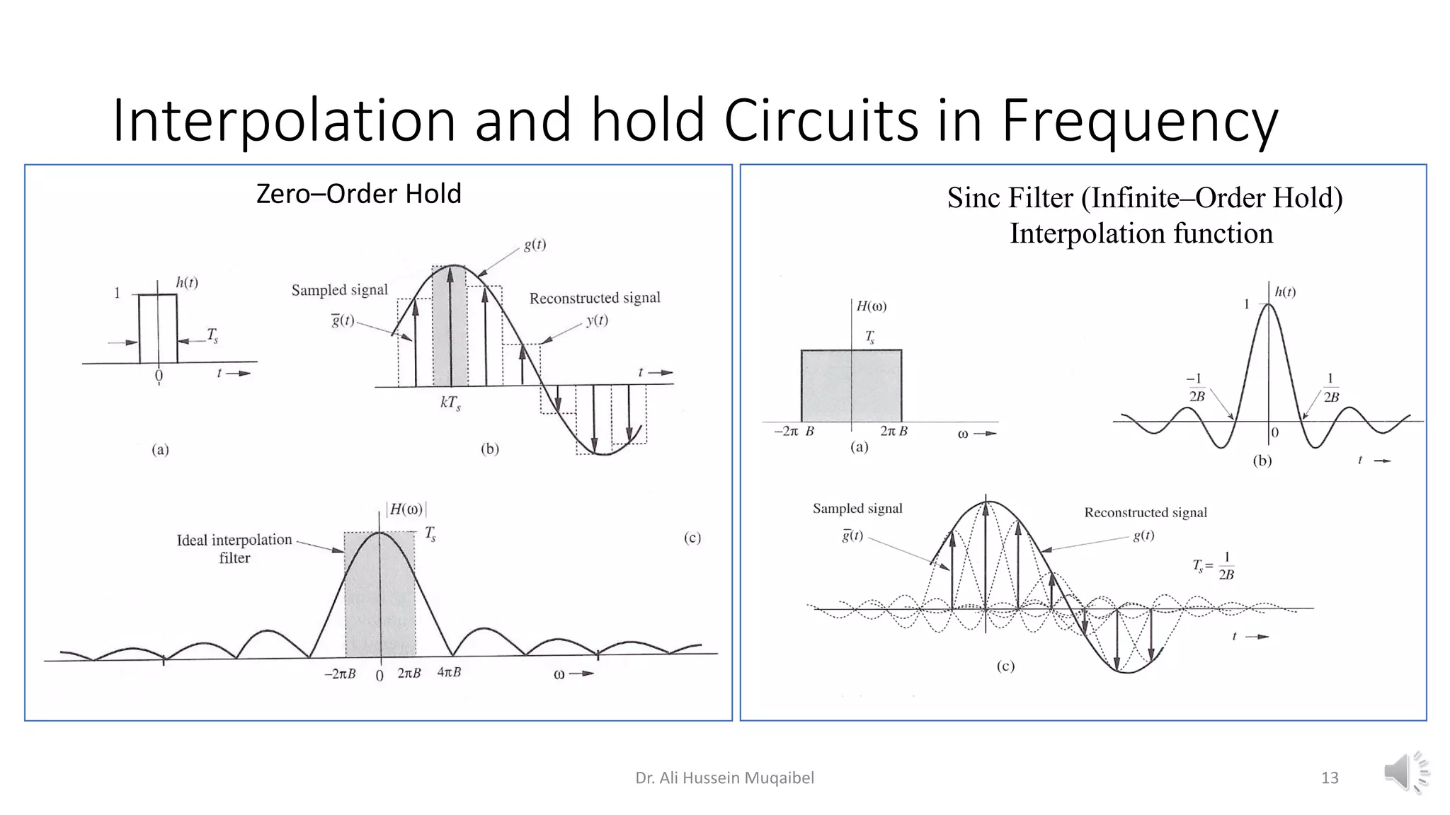
12. Order of Signal Reconstruction (Reconstruction Filters)
Zero–Order Hold
Dr. Ali Hussein Muqaibel
Ts
g(t)
Ts
t
h0(t)
1
Ts
g(t)
1
Ts
t
h1(t)
–Ts
Ts
g(t)
First–Order Hold
–2Ts 2Ts
Ts
–Ts
1
t
hOO(t)
Sinc Filter (Infinite–Order Hold)
Ts
g(t)
12
𝑦 𝑡 = ℎ 𝑡 ∗ ҧ
𝑔 𝑡 = ℎ 𝑡 ∗ [𝑔 𝑡 𝛿𝑇𝑠
𝑡 ]

13. Interpolation and hold Circuits in Frequency
Dr. Ali Hussein Muqaibel 13
Zero–Order Hold Sinc Filter (Infinite–Order Hold)
Interpolation function

14. Practical Sampling Pulses
• Finite width practical pulses
• Because it is periodic, using Fourier
series representation
𝑃𝑇𝑠
= ෍
−∞
+∞
𝐶𝑛𝑒𝑗2𝜋𝑛𝑓𝑠
• Not
𝜹𝑻𝒔
𝒕 =
𝟏
𝑻𝒔
෍
−∞
+∞
𝑒𝑗𝑛2𝜋𝑓𝑠𝑡
Dr. Ali Hussein Muqaibel 14

15. Practical Difficulty in Signal Reconstruction
• To avoid the need for ideal filter 𝑓𝑠 > 2𝐵, we may use a filter with gradual cutoff
characteristics.
• Also we want the filter to be zero outside...(Impossible by Paley-Wiener criterion)
but closely approximated.
Dr. Ali Hussein Muqaibel 15
G()
+2B

2B s s
s
s s
s
A/Ts
...
...
s+2B
s–2B
s+2B
s–2B
LPF for reconstructing the origianl
signal from the sampled signal
Reconstructed Signal
+2B
2B s s
s
s s
s
A/Ts
Ts
Magnitude of LPF should be Ts to cancel
the scaling factor caused by sampling
s > 2(2B)  No interference between Images
