2
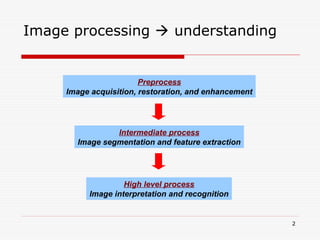
Image processing understanding
Preprocess
Image acquisition, restoration, and enhancement
Intermediate process
Image segmentation and feature extraction
High level process
Image interpretation and recognition
3.
3
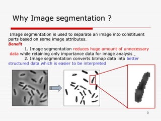
Why Image segmentation?
Image segmentation is used to separate an image into constituent
parts based on some image attributes.
Benefit
1. Image segmentation reduces huge amount of unnecessary
data while retaining only importance data for image analysis
2. Image segmentation converts bitmap data into better
structured data which is easier to be interpreted
4.
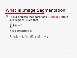
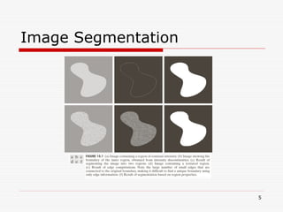
What is ImageSegmentation
It is a process that partitions R(image) into n
sub regions, such that
Ri is a connected set
4
6
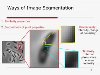
Ways of ImageSegmentation
1. Similarity properties
2. Discontinuity of pixel properties Discontinuity:
Intensity change
at boundary
Similarity:
Internal
pixels share
the same
intensity
7.
7
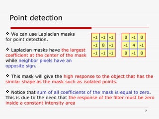
Point detection
Wecan use Laplacian masks
for point detection.
Laplacian masks have the largest
coefficient at the center of the mask
while neighbor pixels have an
opposite sign.
This mask will give the high response to the object that has the
similar shape as the mask such as isolated points.
Notice that sum of all coefficients of the mask is equal to zero.
This is due to the need that the response of the filter must be zero
inside a constant intensity area
-1 -1
-1
8
-1
-1
-1
-1
-1
-1 0
0
4
-1
-1
0
-1
0
8.
8
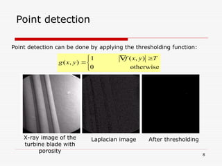
Point detection
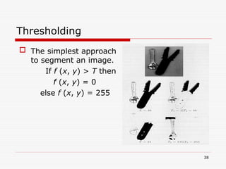
Point detectioncan be done by applying the thresholding function:
otherwise
0
)
,
(
1
)
,
(
T
y
x
f
y
x
g
Laplacian image After thresholding
X-ray image of the
turbine blade with
porosity
9.
9
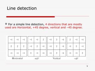
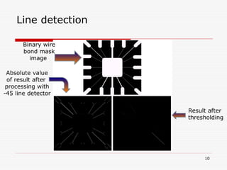
Line detection
Fora simple line detection, 4 directions that are mostly
used are Horizontal, +45 degree, vertical and –45 degree.
11
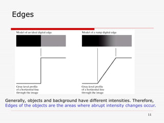
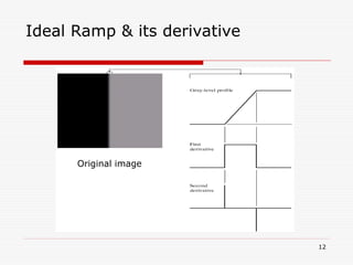
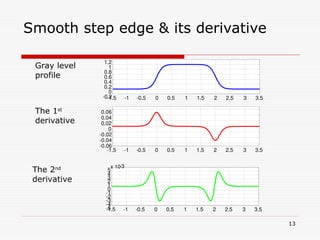
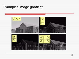
Edges
Generally, objects andbackground have different intensities. Therefore,
Edges of the objects are the areas where abrupt intensity changes occur.
16
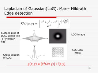
Laplacian of Gaussian(LoG),Marr- Hildrath
Edge detection
2
2
2
2
4
2
2
2
2
)
,
(
y
x
e
y
x
y
x
G
LOG image
5x5 LOG
mask
Surface plot of
LOG, Looks like
a “Mexican
hat”
Cross section
of LOG
17.
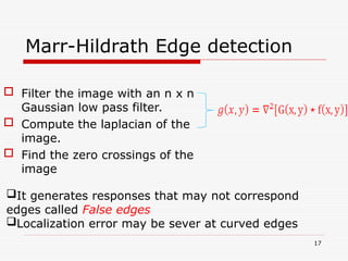
Marr-Hildrath Edge detection
Filter the image with an n x n
Gaussian low pass filter.
Compute the laplacian of the
image.
Find the zero crossings of the
image
17
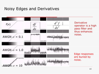
It generates responses that may not correspond
edges called False edges
Localization error may be sever at curved edges
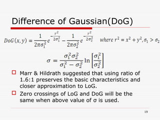
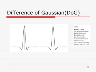
Difference of Gaussian(DoG)
Marr & Hildrath suggested that using ratio of
1.6:1 preserves the basic characteristics and
closer approximation to LoG.
Zero crossings of LoG and DoG will be the
same when above value of σ is used.
19
21
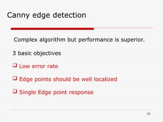
Canny edge detection
Complexalgorithm but performance is superior.
3 basic objectives
Low error rate
Edge points should be well localized
Single Edge point response
22.
22
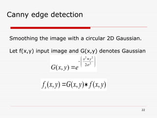
Canny edge detection
Smoothingthe image with a circular 2D Gaussian.
Let f(x,y) input image and G(x,y) denotes Gaussian
2
2
2
2
)
,
(
y
x
e
y
x
G
)
,
(
)
,
(
)
,
( y
x
f
y
x
G
y
x
fs
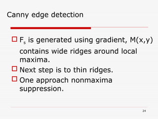
Fs isgenerated using gradient, M(x,y)
contains wide ridges around local
maxima.
Next step is to thin ridges.
One approach nonmaxima
suppression.
24
Canny edge detection
25.
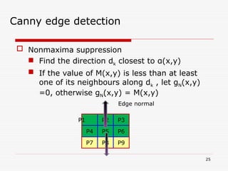
Nonmaxima suppression
Find the direction dk closest to α(x,y)
If the value of M(x,y) is less than at least
one of its neighbours along dk , let gN(x,y)
=0, otherwise gN(x,y) = M(x,y)
25
Canny edge detection
P2 P3
P9
P5
P8
P6
P1
P4
P7
Edge normal
26.
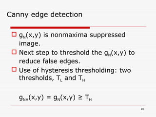
gN(x,y) isnonmaxima suppressed
image.
Next step to threshold the gN(x,y) to
reduce false edges.
Use of hysteresis thresholding: two
thresholds, TL and TH
gNH(x,y) = gN(x,y) ≥ TH
26
Canny edge detection
27.
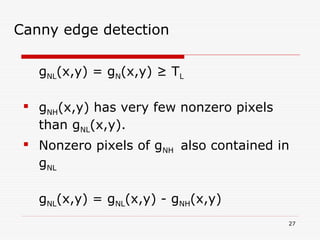
gNL(x,y) = gN(x,y)≥ TL
gNH(x,y) has very few nonzero pixels
than gNL(x,y).
Nonzero pixels of gNH also contained in
gNL
gNL(x,y) = gNL(x,y) - gNH(x,y)
27
Canny edge detection
28.
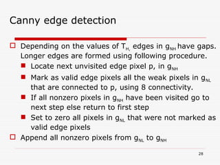
Depending onthe values of TH, edges in gNH have gaps.
Longer edges are formed using following procedure.
Locate next unvisited edge pixel p, in gNH
Mark as valid edge pixels all the weak pixels in gNL
that are connected to p, using 8 connectivity.
If all nonzero pixels in gNH have been visited go to
next step else return to first step
Set to zero all pixels in gNL that were not marked as
valid edge pixels
Append all nonzero pixels from gNL to gNH
28
Canny edge detection
29.
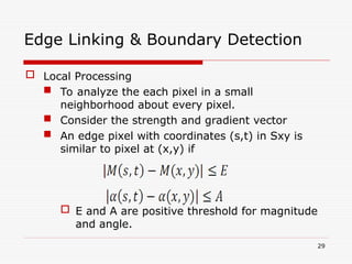
Edge Linking &Boundary Detection
Local Processing
To analyze the each pixel in a small
neighborhood about every pixel.
Consider the strength and gradient vector
An edge pixel with coordinates (s,t) in Sxy is
similar to pixel at (x,y) if
E and A are positive threshold for magnitude
and angle.
29
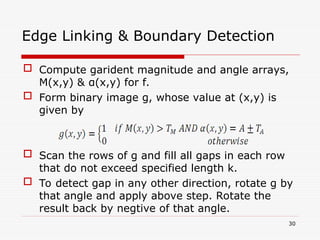
30.
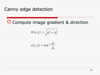
Compute garidentmagnitude and angle arrays,
M(x,y) & α(x,y) for f.
Form binary image g, whose value at (x,y) is
given by
Scan the rows of g and fill all gaps in each row
that do not exceed specified length k.
To detect gap in any other direction, rotate g by
that angle and apply above step. Rotate the
result back by negtive of that angle.
30
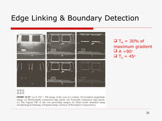
Edge Linking & Boundary Detection
31.
31
TM =30% of
maximum gradient
A =90o
TA = 45o
Edge Linking & Boundary Detection
32.
Given npoints, we want to find subsets of these
points that lie on straight lines.
Find all lines determined by every pair of
points
Then find all subsets of points that are close
to particular lines
Approach involves finding n(n-1)/2 = n2
lines
and then n3
comparisons.
Alternative approach proposed by Hough[1962].
32
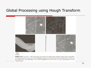
Global Processing using Hough Transform
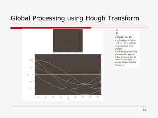
33.
33
Global Processing usingHough Transform
xy plane is transformed to ab plane(Parameter space).
All the points on the line have lines in parameter space
that intersect at (a’, b’).
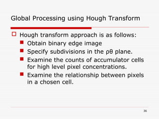
Hough transformapproach is as follows:
Obtain binary edge image
Specify subdivisions in the ρθ plane.
Examine the counts of accumulator cells
for high level pixel concentrations.
Examine the relationship between pixels
in a chosen cell.
36
Global Processing using Hough Transform
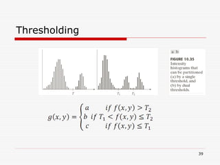
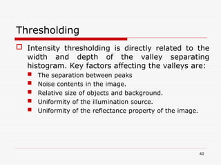
Intensity thresholdingis directly related to the
width and depth of the valley separating
histogram. Key factors affecting the valleys are:
The separation between peaks
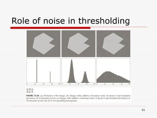
Noise contents in the image.
Relative size of objects and background.
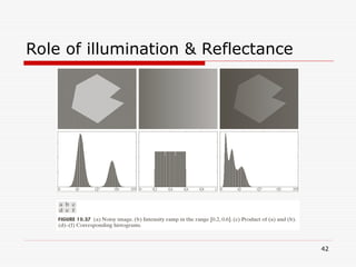
Uniformity of the illumination source.
Uniformity of the reflectance property of the image.
40
Thresholding
Basic Global thresholding
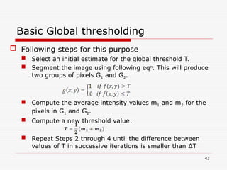
Following steps for this purpose
Select an initial estimate for the global threshold T.
Segment the image using following eqn
. This will produce
two groups of pixels G1 and G2.
Compute the average intensity values m1 and m2 for the
pixels in G1 and G2.
Compute a new threshold value:
Repeat Steps 2 through 4 until the difference between
values of T in successive iterations is smaller than ∆T
43
44.
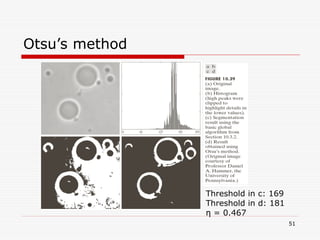
Optimum Global Thresholdingusing “Otsu”
Thresholding may be viewed as decision theory
problem.
Otsu's method tries to maximize between class
variance.
Let L distinct intensity levels in a digital image of
size M x N image.
Suppose, T(k) = k, 0<k<L-1, threshold the input
image in class C1 and C2. C1 consists of all pixels in
the range [0,k] and C2 in the range of [k+1, L-1].
44
45.
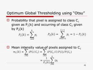
Probability thatpixel is assigned to class C1
given as P1(k) and occurring of class C2 given
by P2(k)
Mean intensity value of pixels assigned to C1
45
Optimum Global Thresholding using “Otsu”
46.
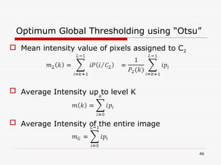
Mean intensityvalue of pixels assigned to C2
Average Intensity up to level K
Average Intensity of the entire image
46
Optimum Global Thresholding using “Otsu”
47.
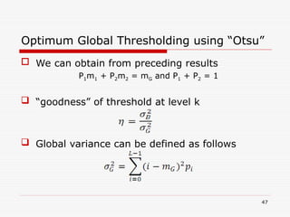
We canobtain from preceding results
P1m1 + P2m2 = mG and P1 + P2 = 1
“goodness” of threshold at level k
Global variance can be defined as follows
47
Optimum Global Thresholding using “Otsu”
48.
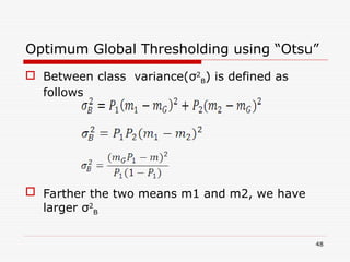
Between classvariance(σ2
B) is defined as
follows
Farther the two means m1 and m2, we have
larger σ2
B
48
Optimum Global Thresholding using “Otsu”
49.
σ2
G isConstant and is a measure of separability.
Objective: Determine k which maximizes between
class variance.
Once k* has been obtained, segment the image.
49
Optimum Global Thresholding using “Otsu”
50.
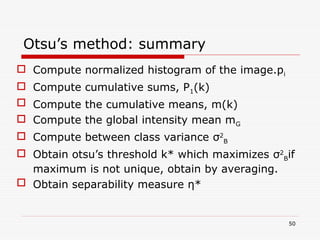
Otsu’s method: summary
Compute normalized histogram of the image.pi
Compute cumulative sums, P1(k)
Compute the cumulative means, m(k)
Compute the global intensity mean mG
Compute between class variance σ2
B
Obtain otsu’s threshold k* which maximizes σ2
Bif
maximum is not unique, obtain by averaging.
Obtain separability measure η*
50
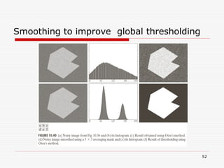
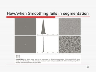
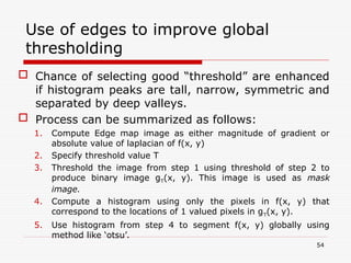
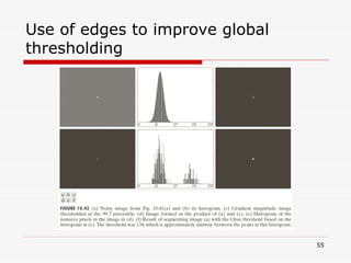
Use of edgesto improve global
thresholding
Chance of selecting good “threshold” are enhanced
if histogram peaks are tall, narrow, symmetric and
separated by deep valleys.
Process can be summarized as follows:
1. Compute Edge map image as either magnitude of gradient or
absolute value of laplacian of f(x, y)
2. Specify threshold value T
3. Threshold the image from step 1 using threshold of step 2 to
produce binary image gT(x, y). This image is used as mask
image.
4. Compute a histogram using only the pixels in f(x, y) that
correspond to the locations of 1 valued pixels in gT(x, y).
5. Use histogram from step 4 to segment f(x, y) globally using
method like ‘otsu’.
54
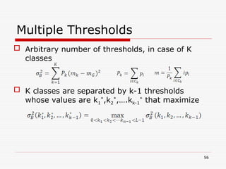
Multiple Thresholds
Arbitrarynumber of thresholds, in case of K
classes
K classes are separated by k-1 thresholds
whose values are k1
*
,k2
*
,….kk-1
*
that maximize
56
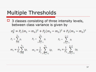
57.
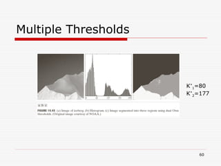
3 classesconsisting of three intensity levels,
between class variance is given by
57
Multiple Thresholds
58.
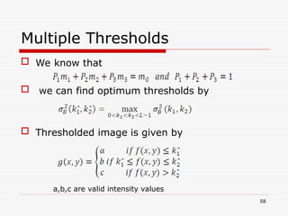
We knowthat
we can find optimum thresholds by
Thresholded image is given by
58
Multiple Thresholds
a,b,c are valid intensity values
59.
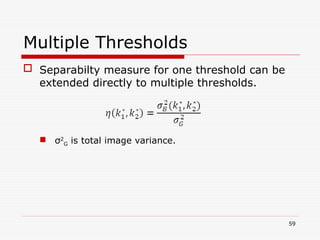
Separabilty measurefor one threshold can be
extended directly to multiple thresholds.
σ2
G is total image variance.
59
Multiple Thresholds
Region based Segmentation
Region growing
It is a procedure that groups pixels into
larger regions based on predefined criteria
for growth.
Start with a set of “seed” points and from
these grow regions by appending to each
seed those nearer pixels that are similar in
criteria to seed.
Criteria depends on the type of image.
61
62.
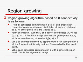
Region growing
Regiongrowing algorithm based on 8 connectivity
is as follows:
Find all connected components in S(x, y) and erode each
connected component to one pixel; label all such pixels found
as 1. All other pixels in S are labeled as 0.
Form an image fQ such that, at a pair of coordinates (x, y), let
fQ(x, y) = 1 if the input image satisfies the given predicate, Q
at those coordinates; otherwise, fQ(x, y) = 0.
Let g be an image formed by appending to each seed point in S
all the 1 valued points in fQ that are 8-connected to that seed
point.
Label each connected component in g with a different region
label. This is the segmented image.
62

![ Given n points, we want to find subsets of these
points that lie on straight lines.
Find all lines determined by every pair of
points
Then find all subsets of points that are close
to particular lines
Approach involves finding n(n-1)/2 = n2
lines
and then n3
comparisons.
Alternative approach proposed by Hough[1962].
32
Global Processing using Hough Transform](https://image.slidesharecdn.com/imagesegmentation-ch10-250904163143-7de0a963/85/Image-process-Image-segmentation-Ch10-ppt-32-320.jpg)


![Optimum Global Thresholding using “Otsu”
Thresholding may be viewed as decision theory
problem.
Otsu's method tries to maximize between class
variance.
Let L distinct intensity levels in a digital image of
size M x N image.
Suppose, T(k) = k, 0<k<L-1, threshold the input
image in class C1 and C2. C1 consists of all pixels in
the range [0,k] and C2 in the range of [k+1, L-1].
44](https://image.slidesharecdn.com/imagesegmentation-ch10-250904163143-7de0a963/85/Image-process-Image-segmentation-Ch10-ppt-44-320.jpg)