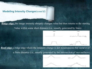
![what is edge detection?
Edges are places in the image with strong intensity contrast (Or) it ‘difference of
intensity between two images (Or) Edges are pixels where image brightness
changes abruptly.
Example:
(a) (b)
Figure 1.1
edge detection: (a) shows [original image] that will be used to find its edge, (b)
shows edge Detection of image using [canny edge detection] method.](https://image.slidesharecdn.com/notesonimageprocessing-160421180107-181118012256/85/Notes-on-image-processing-2-320.jpg)


![Main Steps in Edge Detection
(1) Smoothing: suppress as much noise as possible, without destroying true edges. (Or) it
Make pixel nearest as possible to each other to make image more clearly
Is also called [Blur].
(2)Enhancement: apply differentiation to enhance the quality of edges (sharpening).and apply
some kind of filter that responds strongly at edges for example Take highest
Value of pixel in image and replace it with all pixel to Increase quality of image.
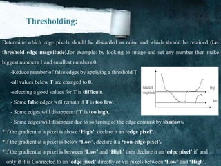
(3)Thresholding: determine which edge pixels should be discarded as noise and which should be
retain (I.e. threshold edge magnitude).
(4) Localization: determine the exact edge location.
** (Sub-pixel resolution): might be required for some applications to estimate the location of an
edge to better than the spacing between pixels.](https://image.slidesharecdn.com/notesonimageprocessing-160421180107-181118012256/85/Notes-on-image-processing-8-320.jpg)
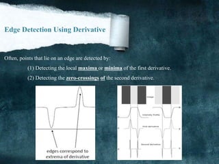
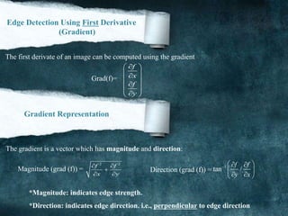
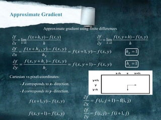
![Edge Detection Using First Derivative
1D functions (not centered at x)
0
( ) ( )
'( ) lim ( 1) ( )
h
f x h f x
f x f x f x
h
(h=1) Mask: [-1 1]
1,0,1Mask M= (Centered at x)
Edge Detection Using Second Derivative
Approximate finding maxima/minima of gradient magnitude by finding places where:
2
( ) 0
2
d f
x
dx
Can’t always find discrete pixels where the second derivative is ((zero)) look for zero-crossing
instead. (See below).
0
'( ) '( )
''( ) lim '( 1) '( )
h
f x h f x
f x f x f x
h
( 2) 2 ( 1) ( )f x f x f x (h=1)
Replace x+1 with x (i.e., centered at x):
''( ) ( 1) 2 ( ) ( 1)f x f x f x f x Mask: [1 -2 1]](https://image.slidesharecdn.com/notesonimageprocessing-160421180107-181118012256/85/Notes-on-image-processing-10-320.jpg)
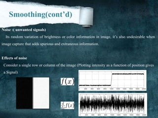
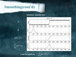
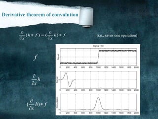
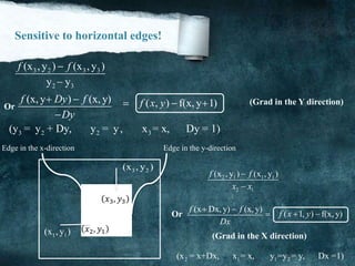
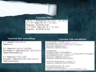
![Smoothing
We will try to suppress as much noise as possible, without smoothing away the meaningful
edges. It make pixel nearest as possible to each other to make image more clearly It’s also
known by [Blur].
But it different than zooming because when you zoom an image using pixel replication and
zooming factor is increased, you saw a blurred image. This image also has less details, but it
is not true blurring. Because in zooming, you add new pixels to an image, which increase
the overall number of pixels in an image, whereas in blurring, the number of pixels of a
normal image and a blurred image remains the same.
Smoothing can be achieved by many ways. The common type of filters that are used to
perform blurring: [1] Mean filter (Box filter).
[2]Weighted average filter.
[3]Gaussian filter.](https://image.slidesharecdn.com/notesonimageprocessing-160421180107-181118012256/85/Notes-on-image-processing-12-320.jpg)
![Thresholding(cont’d)
(a) (b)
(c) Figure 1.5 (d)
Figure 1.5: (a) shows [original image], (b) shows [Fine scale high threshold], (c)
shows [Coarse scale high threshold], (d) shows [coarse scale low threshold].](https://image.slidesharecdn.com/notesonimageprocessing-160421180107-181118012256/85/Notes-on-image-processing-17-320.jpg)
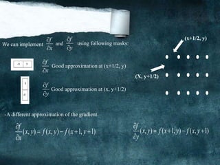
![another Approximation
0 1 2
7 3
6 5 4
[i,j]
a a a
a a
a a a
Consider the arrangement of pixels about the pixel (I, J):
3 x 3 neighborhood:
f
x
f
y
The partial derivatives can be computed by:
2 3 4 0 7 6(a a a ) (a a a )XM c c 6 5 4 0 1 2(a a a ) (a a a )yM c c
The constant c implies the emphasis given to pixels closer to the center of the mask
Roberts Operator
f
x
f
y
= f (i, j) - f )i + 1, j + 1)
= f (i + 1, j)- f (i, j + 1)
This approximation can be implemented by the following masks:
1 0
0 1
0 1
1 0
(Note: Mx and My are approximations at (i + 1/2, j + 1/2))](https://image.slidesharecdn.com/notesonimageprocessing-160421180107-181118012256/85/Notes-on-image-processing-22-320.jpg)
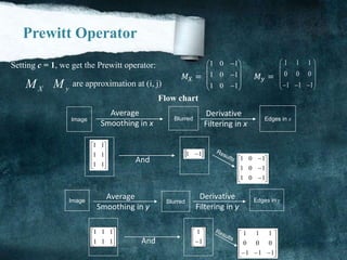
![Edge Detection Steps Using Gradient
A) Smooth the input image ( ( , ) ( , )*G(x, y))F x y f x y
( , )*M ( , )X XF f x y x y
C) ( , )*M ( , )y yF f x y x y
B)
D) Magnitude ( , ) X yx y F F
.
E) Direction
1
( , ) tan (F / F )X yx y
F) IF magnitude ( , ) Tx y , then possible edge point.
(a) (b) (c) (d) (e)
Figure1.6
Figure 1.6:(a) shows [Original image], (b) shows how image represented using [Sobel 3x3],(c) show [Sobel
3x3 grayscale],(d) shows how image represented using [Prewitt 3x3], and (e) shows [Prewitt 3x3 grayscale] .](https://image.slidesharecdn.com/notesonimageprocessing-160421180107-181118012256/85/Notes-on-image-processing-26-320.jpg)
![Marr Hildreth Edge Detector
The derivative operators presented so far are not very useful because they are very
sensitive to noise. To filter the noise before enhancement, Marr and Hildreth proposed a
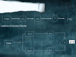
Gaussian Filter, combined with the Laplacian for edge detection. Is the Laplacian of
Gaussian (LoG)?
The fundamental characteristics of LoG edge detector are:
[1] Smooth image by Gaussian filter:
S = G * I
Where: S: is smoothed image.
G: is Gaussian filter represented by
2 2
2
21
( , )
2
x y
G x y e
I: the original image.
[2] Apply Laplacian
2 2
2
2 2
s s s
x y
Note: [ [ ] is used for gradient or derivative.]is used for laplacian](https://image.slidesharecdn.com/notesonimageprocessing-160421180107-181118012256/85/Notes-on-image-processing-27-320.jpg)
![Marr Hildreth Edge Detector
(cont’d)
[3] Deriving the Laplacian of Gaussian (LoG)
2 2 2
( * ) ( )*IS G I G
2 2
2
2 2
22
23
1
(2 )
2
x y
x y
g e
Used in mechanics, electromagnetics, wave theory, quantum mechanics and Laplace equation
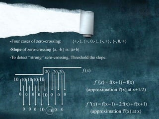
[4] Find zero crossings
(a)Scan along each row, record an edge point at the location of zero-crossing.
(b)Repeat above step along each column.
-Four cases of zero-crossing: {+,-}, {+, 0,-}, {-, +}, {-, 0, +}
-Slope of zero-crossing {a, -b} is: |a+b|
-To detect “strong” zero-crossing, and threshold the slope.
The Separability of LoG
Similar to separability of Gaussian filter two-dimensional Gaussian can be separated into 2
one-dimensional Gaussians.](https://image.slidesharecdn.com/notesonimageprocessing-160421180107-181118012256/85/Notes-on-image-processing-28-320.jpg)
![Steps of Canny edge detector:
Xf yf[1]Compute and
( * ) * *GXf G f G f
x x
( * ) * *Gyf G f G f
y y
Xf yf
G(x, y) is the Gaussian function
2
( , y)
x
G x
2
( , y)
y
G x
Gx
Gx(x, y) is the derivate of (x, y) with respect to x: (x, y) =
Gy
Gy(x, y) is the derivate of (x, y) with respect to y: (x, y) =
[2]Compute the gradient magnitude and direction: Magnitude (I, j) =
2 2
X yf f
[3]Apply non-maxima suppression.
[4]Apply hysteresis thresholding/edge linking.](https://image.slidesharecdn.com/notesonimageprocessing-160421180107-181118012256/85/Notes-on-image-processing-31-320.jpg)
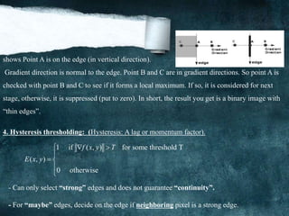
![Hysteresis thresholding uses two thresholds:
-Low threshold 1t -high threshold ht ht 1t(usually = 2 )
1
0 1
0
( , ) definitely an edge
( , ) mayebe an edge,depends on context
( , ) < definitely not an edge
f x y t
t f x y t
f x y t
(a) (b) (c) (d) (e)
Figure 1.7
(a) shows [Original image], (b) shows how image represented using [Grayscale image], (c) show [Gradient
magnitude], (d) shows how image represented using [Thresholded gradient magnitude], and (e) shows
[non-maxima suppression (thinning)].](https://image.slidesharecdn.com/notesonimageprocessing-160421180107-181118012256/85/Notes-on-image-processing-34-320.jpg)


![References
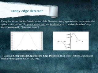
[1] J. F. Canny, .A computational approach to edge detection. IEEE Trans.Pattern Anal.
Machine Intel vol. 8, No. 6, pp. 679.698, Nov. 2007.
[2] Classical feature detection:
URL: http://www.dai.ed.ac.uk/CVonline/LOCAL_COPIES/OWENS/LECT6/node2.html
[3] Edge detection tutorial URL: http://www.pages.drexel.edu/~weg22/edge.html
[4] Canny edge detection tutorial URL: http://www.pages.drexel.edu/~weg22/can_tut.html
[5] Sobel edge detection algorithm URL: http://www.dai.ed.ac.uk/HIPR2/sobel.htm
[6] Gaussian filtering URL: http://robotics.eecs.berkeley.edu/~mayi/imgproc/gademo.html
[7] URL: http://docs.opencv.org/doc/tutorials/imgproc/imgtrans/canny_detector/canny_detector.h
[19] URL: http://www.mathworks.com/help/coder/examples/edge-detection-on-images.html
[20] URL: https://www.youtube.com/watch?v=q6fn-i16h20
[21] URL: https://www.youtube.com/watch?v=q6fn-i16h20
[22] URL: https://www.youtube.com/watch?v=CuOoz0eLmG8
[23] URL: http://northstar-www.dartmouth.edu/doc/idl/html_6.2/Smoothing_an_Image.html
[24] URL: http://en.wikipedia.org/wiki/Canny_edge_detector
[25] URL: http://en.wikipedia.org/wiki/Edge_detection
[26] URL: http://www.mathworks.com/discovery/edge-detection.html](https://image.slidesharecdn.com/notesonimageprocessing-160421180107-181118012256/85/Notes-on-image-processing-40-320.jpg)


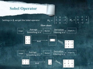
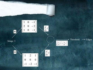
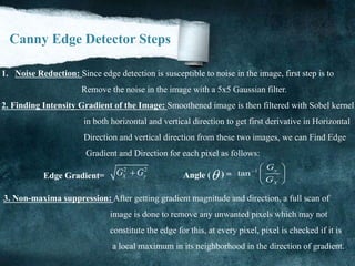
Edge detection is used to identify points in a digital image where the image brightness changes sharply. The key steps are smoothing to reduce noise, enhancing edges through differentiation, thresholding to determine important edges, and localization to find edge positions. Common methods include using the first derivative to find gradients and zero-crossings of the second derivative. Operators like Prewitt and Sobel approximate derivatives with small pixel masks. Edge detection is useful for computer vision tasks by extracting important image features.