CS589-04 Digital ImageProcessing
CS589-04 Digital Image Processing
Lecture 6. Image Segmentation
Lecture 6. Image Segmentation
Spring 2008
Spring 2008
New Mexico Tech
New Mexico Tech
2.
09/13/25 2
Fundamentals
Fundamentals
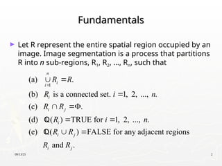
► LetR represent the entire spatial region occupied by an
image. Image segmentation is a process that partitions
R into n sub-regions, R1, R2, …, Rn, such that
1
(a) .
(b) is a connected set. 1, 2, ..., .
(c) .
(d) ( ) TRUE for 1, 2, ..., .
(e) ( ) FALSE for any adjacent regions
and .
n
i
i
i
i j
i
i j
i j
R R
R i n
R R
R i n
R R
R R
09/13/25 6
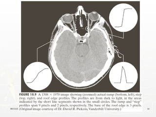
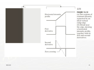
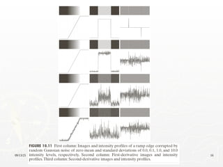
Characteristics ofFirst and Second Order
Characteristics of First and Second Order
Derivatives
Derivatives
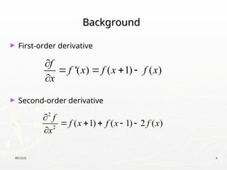
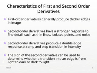
► First-order derivatives generally produce thicker edges
in image
► Second-order derivatives have a stronger response to
fine detail, such as thin lines, isolated points, and noise
► Second-order derivatives produce a double-edge
response at ramp and step transition in intensity
► The sign of the second derivative can be used to
determine whether a transition into an edge is from
light to dark or dark to light
7.
09/13/25 7
Detection ofIsolated Points
Detection of Isolated Points
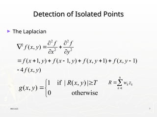
► The Laplacian
2 2
2
2 2
( , )
( 1, ) ( 1, ) ( , 1) ( , 1)
4 ( , )
f f
f x y
x y
f x y f x y f x y f x y
f x y
1 if | ( , ) |
( , )
0 otherwise
R x y T
g x y
9
1
k k
k
R w z
09/13/25 9
Line Detection
LineDetection
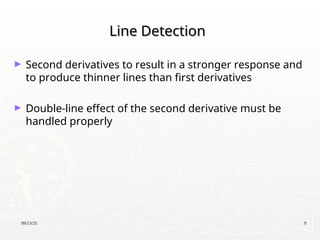
► Second derivatives to result in a stronger response and
to produce thinner lines than first derivatives
► Double-line effect of the second derivative must be
handled properly
09/13/25 11
Detecting Linein Specified Directions
Detecting Line in Specified Directions
► Let R1, R2, R3, and R4 denote the responses of the masks
in Fig. 10.6. If, at a given point in the image, |Rk|>|Rj|,
for all j≠k, that point is said to be more likely associated
with a line in the direction of mask k.
09/13/25 17
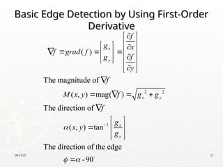
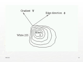
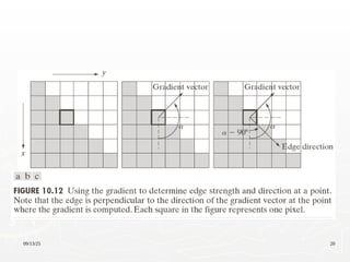
Basic EdgeDetection by Using First-Order
Basic Edge Detection by Using First-Order
Derivative
Derivative
2 2
1
( )
The magnitude of
( , ) mag( )
The direction of
( , ) tan
The direction of the edge
-90
x
y
x y
x
y
f
g x
f grad f
f
g
y
f
M x y f g g
f
g
x y
g
18.
09/13/25 18
Basic EdgeDetection by Using First-Order
Basic Edge Detection by Using First-Order
Derivative
Derivative
Edge normal: ( )
Edge unit normal: / mag( )
x
y
f
g x
f grad f
f
g
y
f f
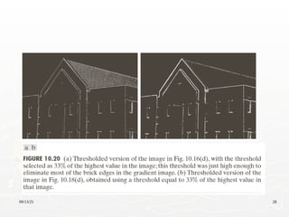
In practice,sometimes the magnitude is approximated by
mag( )= + or mag( )=max | |,| |
f f f f
f f
x y x y
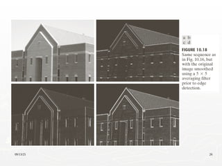
09/13/25 29
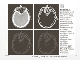
Advanced Techniquesfor Edge Detection
Advanced Techniques for Edge Detection
► The Marr-Hildreth edge detector
2 2
2
2 2 2 2
2 2
2 2 2 2
2 2
2
2 2
2
2 2
2 2
2 2
2 2
2 2
4 2 4 2
2
( , ) , :space constant.
Laplacian of Gaussian (LoG)
( , ) ( , )
( , )
1 1
x y
x y x y
x y x y
G x y e
G x y G x y
G x y
x y
x y
e e
x y
x y
e e
x
2 2
2
2 2
2
4
x y
y
e
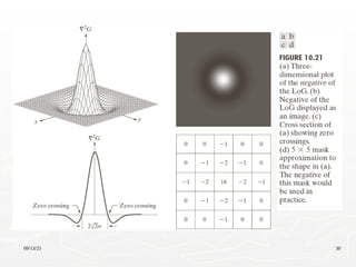
09/13/25 31
Marr-Hildreth Algorithm
Marr-HildrethAlgorithm
1. Filter the input image with an nxn Gaussian lowpass
filter. N is the smallest odd integer greater than or
equal to 6
2. Compute the Laplacian of the image resulting from
step1
3. Find the zero crossing of the image from step 2
2
( , ) ( , ) ( , )
g x y G x y f x y
09/13/25 33
The CannyEdge Detector
The Canny Edge Detector
► Optimal for step edges corrupted by white noise.
► The Objective
1. Low error rate
The edges detected must be as close as possible to the true edge
2. Edge points should be well localized
The edges located must be as close as possible to the true edges
3. Single edge point response
The number of local maxima around the true edge should be
minimum
34.
09/13/25 34
The CannyEdge Detector: Algorithm (1)
The Canny Edge Detector: Algorithm (1)
2 2
2
2
Let ( , ) denote the input image and
( , ) denote the Gaussian function:
( , )
We form a smoothed image, ( , ) by
convolving and :
( , ) ( , ) ( , )
x y
s
s
f x y
G x y
G x y e
f x y
G f
f x y G x y f x y
35.
09/13/25 35
The CannyEdge Detector: Algorithm(2)
The Canny Edge Detector: Algorithm(2)
2 2
Compute the gradient magnitude and direction (angle):
( , )
and
( , ) arctan( / )
where / and /
Note: any of the filter mask pairs in Fig.10.14 can be u
x y
y x
x s y s
M x y g g
x y g g
g f x g f y
sed
to obtain and
x y
g g
36.
09/13/25 36
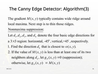
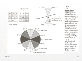
The CannyEdge Detector: Algorithm(3)
The Canny Edge Detector: Algorithm(3)
1 2 3 4
The gradient ( , ) typically contains wide ridge around
local maxima. Next step is to thin those ridges.
Nonmaxima suppression:
Let , , , and denote the four basic edge directions for
a 3 3 regi
M x y
d d d d
o
on: horizontal, -45 ,vertical,+45 ,respectively.
1. Find the direction that is closest to ( , ).
2. If the value of ( , ) is less than at least one of its two
neighbors along , let ( , ) 0
k
k N
d x y
M x y
d g x y
(suppression);
otherwise, let ( , ) ( , )
N
g x y M x y
09/13/25 38
The CannyEdge Detector: Algorithm(4)
The Canny Edge Detector: Algorithm(4)
The final operation is to threshold ( , ) to reduce
false edge points.
Hysteresis thresholding:
( , ) ( , )
( , ) ( , )
and
( , ) ( ,
N
NH N H
NL N L
NL NL
g x y
g x y g x y T
g x y g x y T
g x y g x
) ( , )
NH
y g x y
39.
09/13/25 39
The CannyEdge Detector: Algorithm(5)
The Canny Edge Detector: Algorithm(5)
Depending on the value of , the edges in ( , )
typically have gaps. Longer edges are formed using
the following procedure:
(a). Locate the next unvisited edge pixel, , in ( , ).
(b). Mark as vali
H NH
NH
T g x y
p g x y
d edge pixel all the weak pixels in ( , )
that are connected to using 8-connectivity.
(c). If all nonzero pixel in ( , ) have been visited go to
step (d), esle return to (a).
(d). Set
NL
NH
g x y
p
g x y
to zero all pixels in ( , ) that were not marked as
valid edge pixels.
NL
g x y
40.
09/13/25 40
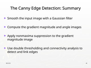
The CannyEdge Detection: Summary
The Canny Edge Detection: Summary
► Smooth the input image with a Gaussian filter
► Compute the gradient magnitude and angle images
► Apply nonmaxima suppression to the gradient
magnitude image
► Use double thresholding and connectivity analysis to
detect and link edges
09/13/25 45
Edge Linkingand Boundary Detection
Edge Linking and Boundary Detection
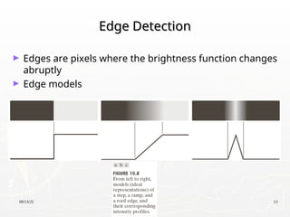
► Edge detection typically is followed by linking
algorithms designed to assemble edge pixels into
meaningful edges and/or region boundaries
► Three approaches to edge linking
Local processing
Regional processing
Global processing
46.
09/13/25 46
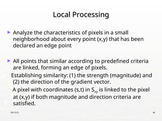
Local Processing
LocalProcessing
► Analyze the characteristics of pixels in a small
neighborhood about every point (x,y) that has been
declared an edge point
► All points that similar according to predefined criteria
are linked, forming an edge of pixels.
Establishing similarity: (1) the strength (magnitude) and
(2) the direction of the gradient vector.
A pixel with coordinates (s,t) in Sxy is linked to the pixel
at (x,y) if both magnitude and direction criteria are
satisfied.
47.
09/13/25 47
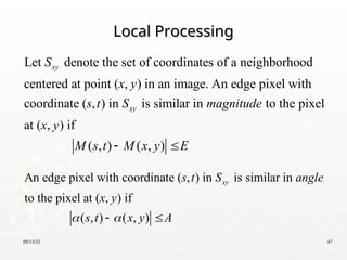
Local Processing
LocalProcessing
Let denote the set of coordinates of a neighborhood
centered at point ( , ) in an image. An edge pixel with
coordinate ( , ) in is similar in to the pixel
at ( , ) if
( ,
xy
xy
S
x y
s t S magnitude
x y
M s ) ( , )
t M x y E
An edge pixel with coordinate ( , ) in is similar in
to the pixel at ( , ) if
( , ) ( , )
xy
s t S angle
x y
s t x y A
48.
09/13/25 48
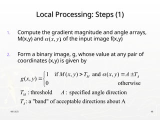
Local Processing:Steps (1)
Local Processing: Steps (1)
1. Compute the gradient magnitude and angle arrays,
M(x,y) and , of the input image f(x,y)
2. Form a binary image, g, whose value at any pair of
coordinates (x,y) is given by
( , )
x y
1 if ( , ) and ( , )
( , )
0 otherwise
: threshold : specified angle direction
: a "band" of acceptable directions about A
M A
M
A
M x y T x y A T
g x y
T A
T
49.
09/13/25 49
Local Processing:Steps (2)
Local Processing: Steps (2)
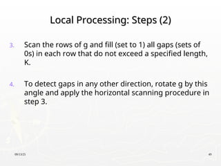
3. Scan the rows of g and fill (set to 1) all gaps (sets of
0s) in each row that do not exceed a specified length,
K.
4. To detect gaps in any other direction, rotate g by this
angle and apply the horizontal scanning procedure in
step 3.
09/13/25 51
Regional Processing
RegionalProcessing
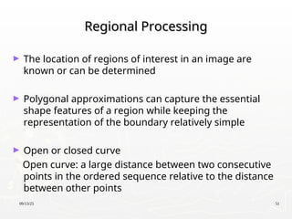
► The location of regions of interest in an image are
known or can be determined
► Polygonal approximations can capture the essential
shape features of a region while keeping the
representation of the boundary relatively simple
► Open or closed curve
Open curve: a large distance between two consecutive
points in the ordered sequence relative to the distance
between other points
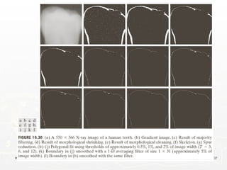
09/13/25 53
Regional Processing:Steps
Regional Processing: Steps
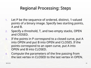
1. Let P be the sequence of ordered, distinct, 1-valued
points of a binary image. Specify two starting points,
A and B.
2. Specify a threshold, T, and two empty stacks, OPEN
and ClOSED.
3. If the points in P correspond to a closed curve, put A
into OPEN and put B into OPEN and CLOSES. If the
points correspond to an open curve, put A into
OPEN and B into CLOSED.
4. Compute the parameters of the line passing from
the last vertex in CLOSED to the last vertex in OPEN.
54.
09/13/25 54
Regional Processing:Steps
Regional Processing: Steps
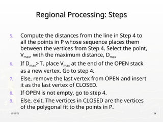
5. Compute the distances from the line in Step 4 to
all the points in P whose sequence places them
between the vertices from Step 4. Select the point,
Vmax, with the maximum distance, Dmax
6. If Dmax> T, place Vmax at the end of the OPEN stack
as a new vertex. Go to step 4.
7. Else, remove the last vertex from OPEN and insert
it as the last vertex of CLOSED.
8. If OPEN is not empty, go to step 4.
9. Else, exit. The vertices in CLOSED are the vertices
of the polygonal fit to the points in P.
09/13/25 58
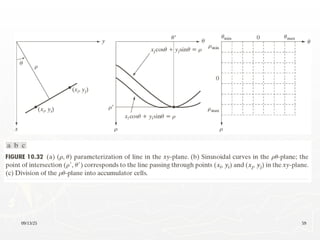
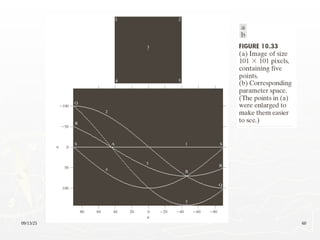
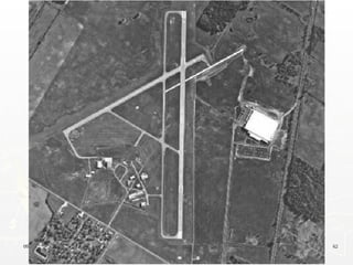
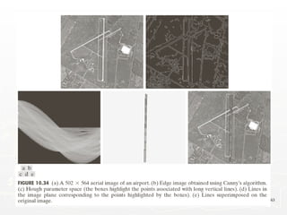
Global ProcessingUsing the Hough
Global Processing Using the Hough
Transform
Transform
► “The Hough transform is a general technique for
identifying the locations and orientations of certain
types of features in a digital image. Developed by Paul
Hough in 1962 and patented by IBM, the transform
consists of parameterizing a description of a feature at
any given location in the original image’s space. A mesh
in the space defined by these parameter is then
generated, and at each mesh point a value is
accumulated, indicating how well an object generated
by the parameters defined at that point fits the given
image. Mesh points that accumulate relatively larger
values then describe features that may be projected
back onto the image, fitting to some degree the
features actually present in the image.”
http://planetmath.org/encyclopedia/HoughTransform.html
09/13/25 61
Edge-linking Basedon the Hough
Edge-linking Based on the Hough
Transform
Transform
1. Obtain a binary edge image
2. Specify subdivisions in
3. Examine the counts of the accumulator cells for high
pixel concentrations
4. Examine the relationship between pixels in chosen
cell
plane
09/13/25 64
Thresholding
Thresholding
1 if( , ) (object point)
( , )
0 if ( , ) (background point)
:global thresholding
f x y T
g x y
f x y T
T
2
1 2
1
Multiple thresholding
if ( , )
( , ) if ( , )
if ( , )
a f x y T
g x y b T f x y T
c f x y T
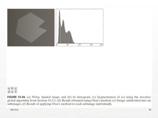
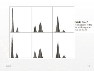
09/13/25 66
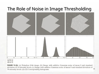
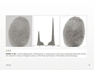
The Roleof Noise in Image Thresholding
The Role of Noise in Image Thresholding
67.
09/13/25 67
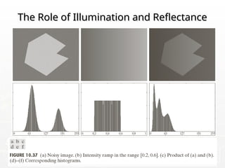
The Roleof Illumination and Reflectance
The Role of Illumination and Reflectance
68.
09/13/25 68
Basic GlobalThresholding
Basic Global Thresholding
1. Select an initial estimate for the global threshold, T.
2. Segment the image using T. It will produce two groups of pixels:
G1 consisting of all pixels with intensity values > T and G2
consisting of pixels with values T.
3. Compute the average intensity values m1 and m2 for the pixels in
G1 and G2, respectively.
4. Compute a new threshold value.
5. Repeat Steps 2 through 4 until the difference between values of T
in successive iterations is smaller than a predefined parameter
.
T
1
1 2
2
T m m
09/13/25 70
Optimum GlobalThresholding Using Otsu’s
Optimum Global Thresholding Using Otsu’s
Method
Method
► Principle: maximizing the between-class variance
1
0
Let {0, 1, 2, ..., -1} denote the distinct intensity levels
in a digital image of size pixels, and let denote the
number of pixels with intensity .
/ and 1
i
L
i i i
i
L L
M N n
i
p n MN p
1 2
is a threshold value, [0, ], [ 1, -1]
k C k C k L
1
1 2 1
0 1
( ) and ( ) 1 ( )
k L
i i
i i k
P k p P k p P k
71.
09/13/25 71
Optimum GlobalThresholding Using Otsu’s
Optimum Global Thresholding Using Otsu’s
Method
Method
1
1 1
0 0
1
The mean intensity value of the pixels assigned to class
C is
1
( ) ( / )
( )
k k
i
i i
m k iP i C ip
P k
2
1 1
2 2
1 1
2
The mean intensity value of the pixels assigned to class
C is
1
( ) ( / )
( )
L L
i
i k i k
m k iP i C ip
P k
1 1 2 2 (Global mean value)
G
Pm P m m
72.
09/13/25 72
Optimum GlobalThresholding Using Otsu’s
Optimum Global Thresholding Using Otsu’s
Method
Method
2
2 2 2
1 1 2 2
2
1 2 1 2
2
1 1 1
1 1
2
1
1 1
Between-class variance, is defined as
( ) ( )
= ( )
=
(1 )
=
(1 )
B
B G G
G
G
P m m P m m
PP m m
m P m P
P P
m P m
P P
73.
09/13/25 73
Optimum GlobalThresholding Using Otsu’s
Optimum Global Thresholding Using Otsu’s
Method
Method
2 2 2
0 1
The optimum threshold is the value, k*, that maximizes
( *), ( *) max ( )
B B B
k L
k k k
1 if ( , ) *
( , )
0 if ( , ) *
f x y k
g x y
f x y k
2
2
Separability measure B
G
74.
09/13/25 74
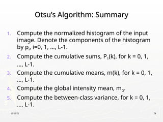
Otsu’s Algorithm:Summary
Otsu’s Algorithm: Summary
1. Compute the normalized histogram of the input
image. Denote the components of the histogram
by pi, i=0, 1, …, L-1.
2. Compute the cumulative sums, P1(k), for k = 0, 1,
…, L-1.
3. Compute the cumulative means, m(k), for k = 0, 1,
…, L-1.
4. Compute the global intensity mean, mG.
5. Compute the between-class variance, for k = 0, 1,
…, L-1.
75.
09/13/25 75
Otsu’s Algorithm:Summary
Otsu’s Algorithm: Summary
6. Obtain the Otsu’s threshold, k*.
7. Obtain the separability measure.
09/13/25 77
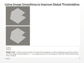
Using ImageSmoothing to Improve Global Thresholding
Using Image Smoothing to Improve Global Thresholding
78.
09/13/25 78
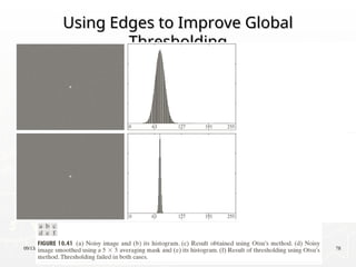
Using Edgesto Improve Global
Using Edges to Improve Global
Thresholding
Thresholding
79.
09/13/25 79
Using Edgesto Improve Global
Using Edges to Improve Global
Thresholding
Thresholding
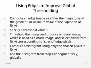
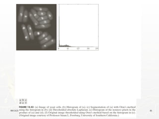
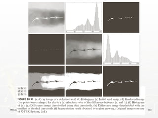
1. Compute an edge image as either the magnitude of
the gradient, or absolute value of the Laplacian of
f(x,y)
2. Specify a threshold value T
3. Threshold the image and produce a binary image,
which is used as a mask image; and select pixels from
f(x,y) corresponding to “strong” edge pixels
4. Compute a histogram using only the chosen pixels in
f(x,y)
5. Use the histogram from step 4 to segment f(x,y)
globally
09/13/25 82
Multiple Thresholds
MultipleThresholds
1 2
2
2
1
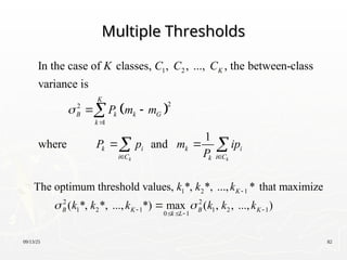
In the case of classes, , , ..., , the between-class
variance is
1
where and
k k
K
K
B k k G
k
k i k i
i C i C
k
K C C C
P m m
P p m ip
P
1 2 1
2 2
1 2 1 1 2 1
0 1
The optimum threshold values, *, *, ..., * that maximize
( *, *, ..., *) max ( , , ..., )
K
B K B K
k L
k k k
k k k k k k
09/13/25 84
Variable Thresholding:Image Partitioning
Variable Thresholding: Image Partitioning
► Subdivide an image into nonoverlapping rectangles
► The rectangles are chosen small enough so that the
illumination of each is approximately uniform.
09/13/25 87
Variable ThresholdingBased on Local
Variable Thresholding Based on Local
Image Properties
Image Properties
Let and denote the standard deviation and mean value
of the set of pixels contained in a neighborhood , centered
at coordinates ( , ) in an image. The local thresholds,
xy xy
xy
xy
m
S
x y
T
If the background is nearly constant,
xy xy
xy xy
a bm
T a bm
1 if ( , )
( , )
0 if ( , )
xy
xy
f x y T
g x y
f x y T
88.
09/13/25 88
Variable ThresholdingBased on Local
Variable Thresholding Based on Local
Image Properties
Image Properties
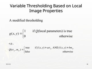
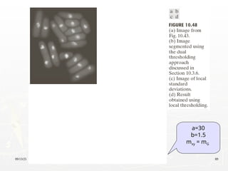
A modified thresholding
1 if (local parameters) is true
( , )
0 otherwise
Q
g x y
. .,
true if ( , ) AND ( , )
( , )
false otherwise
xy xy
xy xy
e g
f x y a f x y bm
Q m
09/13/25 90
Variable ThresholdingUsing Moving
Variable Thresholding Using Moving
Averages
Averages
► Thresholding based on moving averages works well
when the objects are small with respect to the image
size
► Quite useful in document processing
► The scanning (moving) typically is carried out line by
line in zigzag pattern to reduce illumination bias
91.
09/13/25 91
Variable ThresholdingUsing Moving
Variable Thresholding Using Moving
Averages
Averages
1
1
2
Let denote the intensity of the point encountered in
the scanning sequence at step 1. The moving average
(mean intensity) at this new point is given by
1 1
( 1) ( ) (
k
k
i
i k n
z
k
m k z m k
n n
1
1
)
where denotes the number of points used in computing
the average and (1) / , the border of the image were
padded with -1 zeros.
k k
z z
n
m z n
n
92.
09/13/25 92
Variable ThresholdingUsing Moving
Variable Thresholding Using Moving
Averages
Averages
1 if ( , )
( , )
0 if ( , )
xy
xy
xy xy
f x y T
g x y
f x y T
T bm
09/13/25 95
Region-Based Segmentation
Region-BasedSegmentation
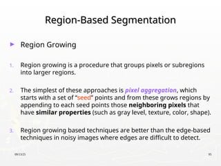
► Region Growing
1. Region growing is a procedure that groups pixels or subregions
into larger regions.
2. The simplest of these approaches is pixel aggregation, which
starts with a set of “seed” points and from these grows regions by
appending to each seed points those neighboring pixels that
have similar properties (such as gray level, texture, color, shape).
3. Region growing based techniques are better than the edge-based
techniques in noisy images where edges are difficult to detect.
96.
09/13/25 96
Region-Based Segmentation
Region-BasedSegmentation
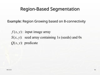
Example:
Example: Region Growing based on 8-connectivity
( , ) : input image array
( , ): seed array containing 1s (seeds) and 0s
( , ): predicate
f x y
S x y
Q x y
97.
09/13/25 97
Region Growingbased on 8-connectivity
1. Find all connected components in ( , ) and erode each
connected components to one pixel; label all such pixels
found as 1. All other pixels in S are labeled 0.
2. Form an image such that, a
Q
S x y
f t a pair of coordinates (x,y),
let ( , ) 1 if the is satisfied otherwise ( , ) 0.
3. Let be an image formed by appending to each seed point
in all the 1-value points in that are 8-con
Q Q
Q
f x y Q f x y
g
S f
nected to that
seed point.
4. Label each connencted component in g with a different region
label. This is the segmented image obtained by region growing.
98.
09/13/25 98
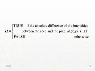
TRUE ifthe absolute difference of the intensities
between the seed and the pixel at (x,y) is T
FALSE otherwise
Q
09/13/25 104
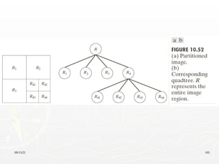
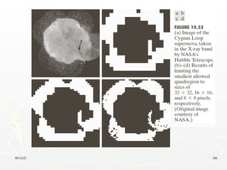
Region Splittingand Merging
Region Splitting and Merging
:entire image :entire image : predicate
1. For any region , If ( ) = FALSE,
we divide the image into quadrants.
2. When no further splitting is possible,
merge any adjacent regi
i
i i
i
R R Q
R Q R
R
ons and
for which ( ) = TRUE.
3. Stop when no further merging is possible.
j k
j k
R R
Q R R
09/13/25 108
Segmentation UsingMorphological
Segmentation Using Morphological
Watersheds
Watersheds
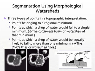
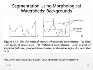
► Three types of points in a topographic interpretation:
Points belonging to a regional minimum
Points at which a drop of water would fall to a single
minimum. (The catchment basin or watershed of
that minimum.)
Points at which a drop of water would be equally
likely to fall to more than one minimum. (The
divide lines or watershed lines.)
Watershed lines
09/13/25 110
Watershed Segmentation:Example
Watershed Segmentation: Example
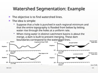
► The objective is to find watershed lines.
► The idea is simple:
Suppose that a hole is punched in each regional minimum and
that the entire topography is flooded from below by letting
water rise through the holes at a uniform rate.
When rising water in distinct catchment basins is about the
merge, a dam is built to prevent merging. These dam
boundaries correspond to the watershed lines.
09/13/25 113
Watershed SegmentationAlgorithm
Watershed Segmentation Algorithm
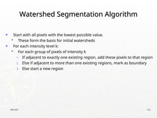
► Start with all pixels with the lowest possible value.
These form the basis for initial watersheds
► For each intensity level k:
For each group of pixels of intensity k
1. If adjacent to exactly one existing region, add these pixels to that region
2. Else if adjacent to more than one existing regions, mark as boundary
3. Else start a new region
114.
09/13/25 114
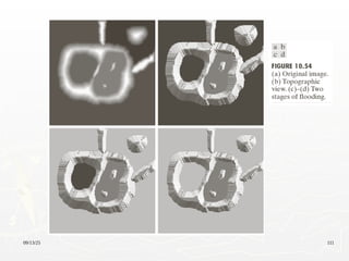
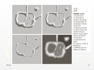
Watershed Segmentation:Examples
Watershed Segmentation: Examples
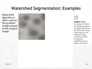
Watershed
algorithm is
often used on
the gradient
image instead
of the original
image.
115.
09/13/25 115
Watershed Segmentation:Examples
Watershed Segmentation: Examples
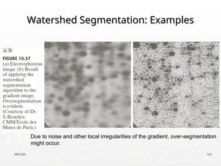
Due to noise and other local irregularities of the gradient, over-segmentation
might occur.
116.
09/13/25 116
Watershed Segmentation:Examples
Watershed Segmentation: Examples
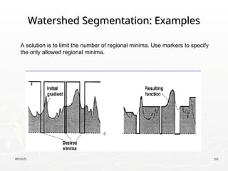
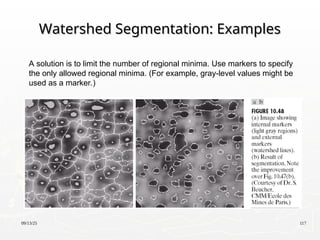
A solution is to limit the number of regional minima. Use markers to specify
the only allowed regional minima.
117.
09/13/25 117
Watershed Segmentation:Examples
Watershed Segmentation: Examples
A solution is to limit the number of regional minima. Use markers to specify
the only allowed regional minima. (For example, gray-level values might be
used as a marker.)
09/13/25 119
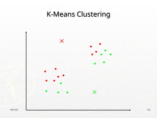
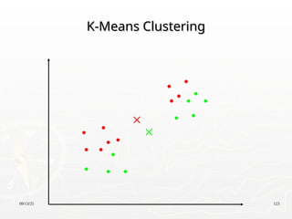
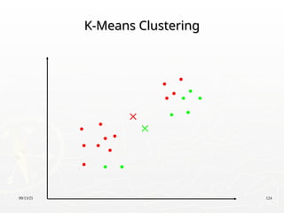
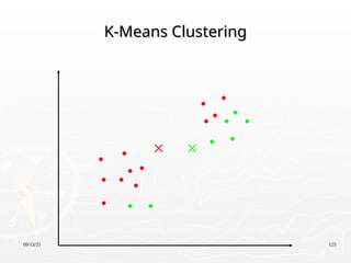
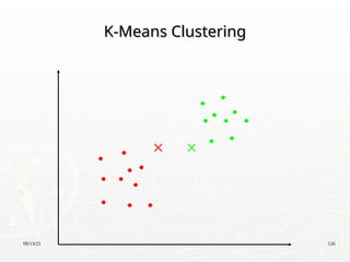
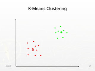
K-means Clustering
K-meansClustering
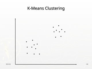
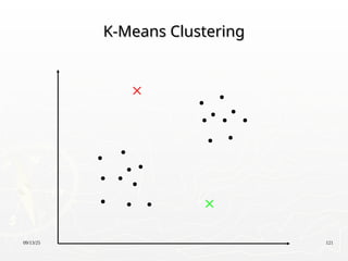
► Partition the data points into K clusters randomly. Find
the centroids of each cluster.
► For each data point:
Calculate the distance from the data point to each cluster.
Assign the data point to the closest cluster.
► Recompute the centroid of each cluster.
► Repeat steps 2 and 3 until there is no further change
in the assignment of data points (or in the centroids).


![09/13/25 70
Optimum Global Thresholding Using Otsu’s
Optimum Global Thresholding Using Otsu’s
Method
Method
► Principle: maximizing the between-class variance
1
0
Let {0, 1, 2, ..., -1} denote the distinct intensity levels
in a digital image of size pixels, and let denote the
number of pixels with intensity .
/ and 1
i
L
i i i
i
L L
M N n
i
p n MN p
1 2
is a threshold value, [0, ], [ 1, -1]
k C k C k L
1
1 2 1
0 1
( ) and ( ) 1 ( )
k L
i i
i i k
P k p P k p P k
](https://image.slidesharecdn.com/lect06-250913161837-1de46abe/85/LectVI______________________________-ppt-70-320.jpg)


![[Deck] What's New in Spark-Iceberg Integration via DSV2.pptx](https://cdn.slidesharecdn.com/ss_thumbnails/deckwhatsnewinspark-icebergintegrationviadsv2-260210005337-25955b12-thumbnail.jpg?width=640&height=640&fit=bounds)


