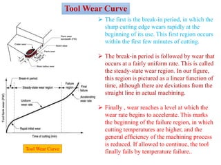
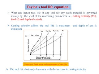
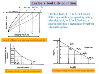
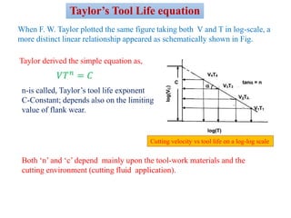
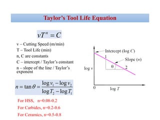
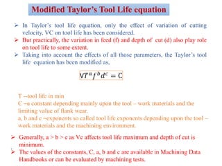
Tool life refers to the amount of time a cutting tool can machine material satisfactorily before needing replacement or reconditioning. It is measured in actual machining time, number of pieces cut, material volume removed, or cutting length. Tool life depends mainly on cutting parameters like velocity, feed, and depth of cut. Initially, tool wear is rapid but then levels off into a steady state wear region before accelerating again towards failure. Taylor's tool life equation models the relationship between cutting velocity and tool life, showing they are inversely proportional. The equation has since been modified to also account for the effects of feed and depth of cut on tool life.

1. Tool Life

2. Tool life generally indicates, the amount of satisfactory performance or
service rendered by a fresh tool or a cutting point till it is declared failed.
In R & D : Actual machining time (period) by which a fresh cutting tool (or
point) satisfactorily works after which it needs replacement or reconditioning.
In industries or shop floor : The length of time of satisfactory service or
amount of acceptable output provided by a fresh tool prior to it is required to
replace or recondition.
Tool life is defined in many ways :
Tool life means,
 no. of pieces of work machined
 total volume of material removed
 total length of cut.
Tool Life

3. i) by loss of tool material in volume or weight, in one life time –generally
applicable for critical tools like grinding wheels.
ii) by grooving and indentation method – in this approximate method wear
depth is measured indirectly by the difference in length of the groove or
the indentation outside and inside the wear area.
iii) using optical microscope fitted with micrometer – very common and
effective method.
Measurement of tool wear

4. Measurement of tool wear
iv) using scanning electron microscope (SEM) – used generally, for detailed
study; both qualitative and quantitative
v) Talysurf profilometer, specially for shallow crater wear.

5.  The first is the break-in period, in which the
sharp cutting edge wears rapidly at the
beginning of its use. This first region occurs
within the first few minutes of cutting.
 The break-in period is followed by wear that
occurs at a fairly uniform rate. This is called
the steady-state wear region. In our figure,
this region is pictured as a linear function of
time, although there are deviations from the
straight line in actual machining.
 Finally , wear reaches a level at which the
wear rate begins to accelerate. This marks
the beginning of the failure region, in which
cutting temperatures are higher, and the
general efficiency of the machining process
is reduced. If allowed to continue, the tool
finally fails by temperature failure..Tool Wear Curve
Tool Wear Curve

6. Taylor’s tool life equation.
 Wear and hence tool life of any tool for any work material is governed
mainly by the level of the machining parameters i.e., cutting velocity (Vc),
feed (f) and depth of cut (d).
 Cutting velocity affects the tool life is maximum and depth of cut is
minimum.
 The tool life obviously decreases with the increase in cutting velocity.
Growth of flank wear and assessment of tool life

7. If the tool lives, T1, T2, T3, T4 etc are
plotted against the corresponding cutting
velocities, Vc1, Vc2, Vc3, Vc4 etc., a
smooth curve like a rectangular hyperbola
is found to appear.
Cutting velocity vs tool life on a log-log scaleCutting velocity – tool life relationship
Taylor’s Tool Life equation
Growth of flank wear and assessment of tool life

8. Taylor derived the simple equation as,
n-is called, Taylor’s tool life exponent
C-Constant; depends also on the limiting
value of flank wear.
When F. W. Taylor plotted the same figure taking both V and T in log-scale, a
more distinct linear relationship appeared as schematically shown in Fig.
Taylor’s Tool Life equation
𝑉𝑇 𝑛 = 𝐶
Both ‘n’ and ‘c’ depend mainly upon the tool-work materials and the
cutting environment (cutting fluid application).
Cutting velocity vs tool life on a log-log scale

9. Taylor’s Tool Life Equation
v – Cutting Speed (m/min)
T – Tool Life (min)
n, C are constants
C – intercept / Taylor’s constant
n – slope of the line / Taylor’s
exponent
n
vT C
1 2
2 1
log log
tan
log log
v v
n
T T


 

For HSS, n=0.08-0.2
For Carbides, n=0.2-0.6
For Ceramics, n=0.5-0.8

10.  In Taylor’s tool life equation, only the effect of variation of cutting
velocity, VC on tool life has been considered.
 But practically, the variation in feed (f) and depth of cut (d) also play role
on tool life to some extent.
 Taking into account the effects of all those parameters, the Taylor’s tool
life equation has been modified as,
T --tool life in min
C ⎯a constant depending mainly upon the tool – work materials and the
limiting value of flank wear.
a, b and c ⎯exponents so called tool life exponents depending upon the tool –
work materials and the machining environment.
 Generally, a > b > c as Vc affects tool life maximum and depth of cut is
minimum.
 The values of the constants, C, a, b and c are available in Machining Data
Handbooks or can be evaluated by machining tests.
.
Modified Taylor’s Tool Life equation
V𝑇 𝑎 𝑓 𝑏 𝑑 𝑐 = C

11. Tutorial –Numerical Problems

12. Taylor’s Tool Life equation-Numerical Problems

13. Merchant’s Circle Diagram-Numerical Problems