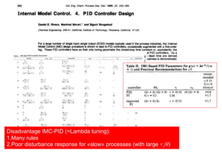
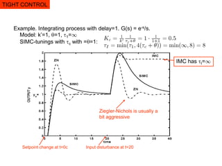
Practical plantwide process
control: PID tuning
Sigurd Skogestad, NTNU
Part 4: PID tuning
Part 2 (4h). PID controller tuning: It pays off to be systematic!
1. Obtaining first-order plus delay models
 Open-loop step response
 From detailed model (half rule)
 From closed-loop setpoint response
2 . Derivation SIMC PID tuning rules
 Controller gain, Integral time, derivative time
3. Special topics
 Integrating processes (level control)
 Other special processes and examples
 When do we need derivative action?
 Near-optimality of SIMC PID tuning rules
 Non PID-control: Is there an advantage in using Smith Predictor? (No)
Examples
Operation: Decision and control layers
cs = y1s
MPC
PID
y2s
RTO
u (valves)
CV=y1; MV=y2s
CV=y2; MV=u
Min J (economics);
MV=y1s
PID controller
 Time domain (“ideal” PID)
 Laplace domain (“ideal”/”parallel” form)
 For our purposes. Simpler with cascade form
 Usually τD=0. Then the two forms are identical.
 Only two parameters left (Kc and τI)
 How difficult can it be to tune???
 Surprisingly difficult without systematic approach!
e
Trans. ASME, 64, 759-768 (Nov. 1942).
Disadvantages Ziegler-Nichols:
1.Aggressive settings
2.No tuning parameter
3.Poor for processes with large time delay (µ)
Comment:
Similar to SIMC for integrating
process with ¿c=0:
Kc = 1/k’ 1/µ
¿I = 4 µ
Disadvantage IMC-PID (=Lambda tuning):
1.Many rules
2.Poor disturbance response for «slow» processes (with large ¿1/µ)
Motivation for developing SIMC
PID tuning rules
1. The tuning rules should be well motivated, and
preferably be model-based and analytically
derived.
2. They should be simple and easy to memorize.
3. They should work well on a wide range of
processes.
SIMC PI tuning rule
1. Approximate process as first-order with delay (e.g., use “half rule”)
 k = process gain
 ¿1 = process time constant
 µ = process delay
2. Derive SIMC tuning rule*:
Reference: S. Skogestad, “Simple analytic rules for model reduction and PID controller design”, J.Proc.Control, Vol. 13, 291-309, 2003
(*) “Probably the best simple PID tuning rules in the world”
c ¸ - : Desired closed-loop response time (tuning parameter)
Open-loop step response
Integral time rule combines well-known rules:
IMC (Lamda-tuning): Same as SIMC for small ¿1 (¿I = ¿1)
Ziegler-Nichols: Similar to SIMC for large ¿1 (if we choose ¿c= 0; aggressive!)
Need a model for tuning
 Model: Dynamic effect of change in input u (MV) on
output y (CV)
 First-order + delay model for PI-control
 Second-order model for PID-control
 Recommend: Use second-order model only if ¿2>µ
MODEL
1. Step response experiment
 Make step change in one u (MV) at a time
 Record the output (s) y (CV)
MODEL, Approach 1A
STEP IN INPUT u
RESULTING OUTPUT y
: Delay - Time where output does not change
1: Time constant - Additional time to reach
63% of final change
k =  y(∞)/ u : Steady-state gain
Δy(∞)
Δu
MODEL, Approach 1A
Step response integrating process
Δy
Δt
MODEL, Approach 1A
Shams’ method: Closed-loop setpoint response
with P-controller with about 20-40% overshoot
Kc0=1.5
Δys=1
Δyu=0.54
Δyp=0.79
tp=4.4
1. OBTAIN DATA IN RED (first overshoot
and undershoot), and then:
tp=4.4, dyp=0.79; dyu=0.54, Kc0=1.5, dys=1
dyinf = 0.45*(dyp + dyu)
Mo =(dyp -dyinf)/dyinf % Mo=overshoot (about 0.3)
b=dyinf/dys
A = 1.152*Mo^2 - 1.607*Mo + 1.0
r = 2*A*abs(b/(1-b))
%2. OBTAIN FIRST-ORDER MODEL:
k = (1/Kc0) * abs(b/(1-b))
theta = tp*[0.309 + 0.209*exp(-0.61*r)]
tau = theta*r
3. CAN THEN USE SIMC PI-rule
Example 2: Get k=0.99, theta =1.68, tau=3.03
Ref: Shamssuzzoha and Skogestad (JPC, 2010)
+ modification by C. Grimholt (Project, NTNU, 2010; see also PID-book 2012)
Δy∞
MODEL, Approach 1B
2. Model reduction of more complicated model
 Start with complicated stable model on the form
 Want to get a simplified model on the form
 Most important parameter is the “effective” delay 
MODEL, Approach 2
MODEL, Approach 2
Example 1
Half rule
MODEL, Approach 2
original
1st-order+delay
MODEL, Approach 2
half rule
2
MODEL, Approach 2
original
1st-order+delay
2nd-order+delay
MODEL, Approach 2
Approximation of zeros
Alternative and improved method forf approximating zeros:
Simple Analytic PID Controller Tuning Rules Revisited
J Lee, W Cho, TF Edgar - Industrial & Engineering Chemistry Research 2014, 53 (13), pp 5038–5047
MODEL, Approach 2
To make these rules more general
(and not only applicable to the
choice c=): Replace  (time
delay) by c (desired closed-loop
response time). (6 places)
c
c
c
c
c
c
Derivation of SIMC-PID tuning rules
 PI-controller (based on first-order model)
 For second-order model add D-action.
For our purposes, simplest with the “series” (cascade) PID-form:
SIMC-tunings
Basis: Direct synthesis (IMC)
Closed-loop response to setpoint change
Idea: Specify desired response:
and from this get the controller. ……. Algebra:
SIMC-tunings
SIMC-tunings
NOTE: Setting the steady-state gain = 1 in T will result in integral action in the controller!
IMC Tuning = Direct Synthesis
Algebra:
SIMC-tunings
Integral time
 Found: Integral time = dominant time constant (I = 1) (IMC-rule)
 Works well for setpoint changes
 Needs to be modified (reduced) for integrating disturbances
Example. “Almost-integrating process” with disturbance at input:
G(s) = e-s/(30s+1)
Original integral time I = 30 gives poor disturbance response
Try reducing it!
g
c
d
y
u
SIMC-tunings
Integral Time
I = 1
Reduce I to this value:
I = 4 (c+) = 8 
SIMC-tunings
Setpoint change at t=0 Input disturbance at t=20
Integral time
 Want to reduce the integral time for “integrating”
processes, but to avoid “slow oscillations” we must require:
 Derivation:
 Setpoint response: Improve (get rid of overshoot) by “pre-
filtering”, y’s = f(s) ys.
SIMC-tunings
Details: See www.nt.ntnu.no/users/skoge/publications/2003/tuningPID Remark 13 II
Conclusion: SIMC-PID Tuning Rules
One tuning parameter: c
SIMC-tunings
Some insights from tuning rules
1. The effective delay θ (which limits the achievable closed-loop
time constant τc) is independent of the dominant process time
constant τ1!
 It depends on τ2/2 (PI) or τ3/2 (PID)
2. Use (close to) P-control for integrating process
 Beware of large I-action (small τI) for level control
3. Use (close to) I-control for fast process (with small time
constant τ1)
4. Parameter variations: For robustness tune at operating point
with maximum value of k’ θ = (k/τ1)θ
SIMC-tunings
Cascade PID -> Ideal PID
SIMC-tunings
Selection of tuning parameter c
Two main cases
1. TIGHT CONTROL: Want “fastest possible
control” subject to having good robustness
• Want tight control of active constraints (“squeeze and shift”)
2. SMOOTH CONTROL: Want “slowest possible
control” subject to acceptable disturbance rejection
• Want smooth control if fast setpoint tracking is not required, for
example, levels and unconstrained (“self-optimizing”) variables
• THERE ARE ALSO OTHER ISSUES: Input
saturation etc.
TIGHT CONTROL:
SMOOTH CONTROL:
SIMC-tunings
TIGHT CONTROL
Typical closed-loop SIMC responses with the choice c=
TIGHT CONTROL
Example. Integrating process with delay=1. G(s) = e-s/s.
Model: k’=1, =1, 1=1
SIMC-tunings with c with ==1:
IMC has I=1
Ziegler-Nichols is usually a
bit aggressive
Setpoint change at t=0c Input disturbance at t=20
TIGHT CONTROL
1. Approximate as first-order model with k=1, 1 = 1+0.1=1.1, =0.1+0.04+0.008 = 0.148
Get SIMC PI-tunings (c=): Kc = 1 ¢ 1.1/(2¢ 0.148) = 3.71, I=min(1.1,8¢ 0.148) = 1.1
2. Approximate as second-order model with k=1, 1 = 1, 2=0.2+0.02=0.22, =0.02+0.008 = 0.028
Get SIMC PID-tunings (c=): Kc = 1 ¢ 1/(2¢ 0.028) = 17.9, I=min(1,8¢ 0.028) = 0.224, D=0.22
TIGHT CONTROL
Tuning for smooth control
Will derive Kc,min. From this we can get c,max using SIMC tuning rule
SMOOTH CONTROL
 Tuning parameter: c = desired closed-loop response time
 Selecting c= (“tight control”) is reasonable for cases with a relatively large
effective delay 
 Other cases: Select c >  for
 slower control
 smoother input usage
 less disturbing effect on rest of the plant
 less sensitivity to measurement noise
 better robustness
 Question: Given that we require some disturbance rejection.
 What is the largest possible value for c ?
 Or equivalently: The smallest possible value for Kc?
S. Skogestad, ``Tuning for smooth PID control with acceptable disturbance rejection'', Ind.Eng.Chem.Res, 45 (23), 7817-7822 (2006).
Closed-loop disturbance rejection
d0
ymax
-d0
-ymax
SMOOTH CONTROL
Kc
u
Minimum controller gain for PI-and PID-control:
min |c(j)| = Kc
SMOOTH CONTROL
Rule: Min. controller gain for
acceptable disturbance rejection:
Kc ¸ |ud|/|ymax|
often ~1 (in span-scaled variables)
SMOOTH CONTROL
|ymax| = allowed deviation for output (CV)
|ud| = required change in input (MV) for disturbance rejection (steady state)
= observed change (movement) in input from historical data
Rule: Kc ¸ |ud|/|ymax|
 Exception to rule: Can have lower Kc if
disturbances are handled by the integral action.
 Disturbances must occur at a frequency lower than 1/I
 Applies to: Process with short time constant (1 is small)
and no delay ( ¼ 0).
 For example, flow control
 Then I = 1 is small so integral action is “large”
SMOOTH CONTROL
Summary: Tuning of easy loops
 Easy loops: Small effective delay ( ¼ 0), so closed-
loop response time c (>> ) is selected for “smooth
control”
 ASSUME VARIABLES HAVE BEEN SCALED WITH
RESPECT TO THEIR SPAN SO THAT |u0/ymax| = 1
(approx.).
 Flow control: Kc=0.2, I = 1 = time constant valve
(typically, 2 to 10s; close to pure integrating!)
 Level control: Kc=2 (and no integral action)
 Other easy loops (e.g. pressure): Kc = 2, I = min(4c, 1)
 Note: Often want a tight pressure control loop (so may have
Kc=10 or larger)
SMOOTH CONTROL
Conclusion PID tuning
S IM C tu n in g ru le s
1 . Tig h t c o ntro l: Se le ct c=  co rres p o n d in g to
2 . S m o oth c o ntro l. S e lect Kc ¸
N o te : H a vin g s e le cte d K c (or c ), th e inte g ra l tim e I sh o u ld b e
s e lec te d a s g ive n a b o ve
3. Derivative time: Only for dominant second-order processes
PID: More (Special topics)
1. Integrating processes (level control)
2. Other special processes and examples
3. When do we need derivative action?
4. Near-optimality of SIMC PID tuning rules
5. Non PID-control: Is there an advantage in using Smith
Predictor? (No)
April 4-8, 2004 KFUPM-Distillation Control Course 46
1. Application of smooth control
 Averaging level control
V
q
LC
Reason for having tank is to smoothen disturbances in concentration and flow.
Tight level control is not desired: gives no “smoothening” of flow disturbances.
SMOOTH CONTROL LEVEL CONTROL
If you insist on integral action
then this value avoids cycling
Proof: 1. Let
|u0| = |q0| – expected flow change [m3/s] (input disturbance)
|ymax| = |Vmax| - largest allowed variation in level [m3]
Minimum controller gain for acceptable disturbance rejection:
Kc ¸ Kc,min = |u0|/|ymax| = |q0| / |Vmax|
2. From the material balance (dV/dt = q – qout), the model is g(s)=k’/s with k’=1.
Select Kc=Kc,min. SIMC-Integral time for integrating process:
I = 4 / (k’ Kc) = 4 |Vmax| / | q0| = 4 ¢ residence time
provided tank is nominally half full and q0 is equal to the nominal flow.
More on level control
 Level control often causes problems
 Typical story:
 Level loop starts oscillating
 Operator detunes by decreasing controller gain
 Level loop oscillates even more
 ......
 ???
 Explanation: Level is by itself unstable and
requires control.
LEVEL CONTROL
Level control: Can have both
fast and slow oscillations
 Slow oscillations (Kc too low): P > 3¿I
 Fast oscillations (Kc too high): P < 3¿I
Here: Consider the less common slow oscillations
LEVEL CONTROL
How avoid oscillating levels?
LEVEL CONTROL
• S im p le st: U se P -c o n tro l o n ly (n o in te g ra l a c tio n )
• If yo u in s is t o n in te g ra l a c tio n , th e n m a k e su re
th e c o n tro lle r g a in is su ffic ie n tly la rg e
• If yo u h a ve a le ve l lo o p th a t is o sc illa tin g th e n
u se S ig u rd s ru le (c an be d erive d):
T o a vo id o sc illatio ns , inc re as e K c ¢I by fa cto r
f= 0 .1 ¢(P 0/I0)2
w h e re
P 0 = p e rio d o f o sc illatio ns [s ]
I0 = o rig ina l inte gra l tim e [s]
0.1 ¼ 1/2
Case study oscillating level
 We were called upon to solve a problem with
oscillations in a distillation column
 Closer analysis: Problem was oscillating reboiler
level in upstream column
 Use of Sigurd’s rule solved the problem
LEVEL CONTROL
LEVEL CONTROL
One tuning parameter: c
SIMC-tunings
2. Some special cases
Another special case: IPZ process
 IPZ-process may represent response from steam flow to pressure
 Rule T2:
 SIMC-tunings
These tunings turn out to be almost identical to the tunings given on page 104-106 in the Ph.D.
thesis by O. Slatteke, Lund Univ., 2006 and K. Forsman, "Reglerteknik for processindustrien",
Studentlitteratur, 2005.
SIMC-tunings
Note: Derivative action is commonly used for temperature control loops.
Select D equal to 2 = time constant of temperature sensor
3. Derivative action?
Time delay process: Setpoint and disturbance responses same + input response same
θ=1
Optimal PI*
Pure time delay process: “Minor”
improvement by adding D-action*
* D-action (ID-control) is equivalent to PI-control (with ¿ >0)
= I-control
Pure time delay process
) Two alternative “Improved SIMC”-rules
Alt. 1. Improved PI-rule (iSIMC-PI): Add θ/3 to 1
Alt. 2. Improved PID-rule (iSIMC-PID): Add θ/3 to 2
iSIMC-PI and iSIMC-PID are identical for pure delay process (¿1=0)
iSIMC-PID is better for integrating process
Integrating process
0 10 20 30 40
0
1
2
3
op t P I D
SI M C P I
i SI M C P I D
op t P I
do di
G(s) = 1
s
e− s
Time, t
Out
put
s,
y
0 10 20 30 40
− 1.5
− 1
− 0.5
0
0.5
op t P I D
op t P I
S
I
M
C
P
I
i SI M C P I D
Time, t
Input
s,
u
 Multiobjective. Tradeoff between
 Output performance
 Robustness
 Input usage
 Noise sensitivity
High controller gain (“tight control”)
Low controller gain (“smooth control”)
• Quantification
– Output performance:
• Rise time, overshoot, settling time
• IAE or ISE for setpoint/disturbance
– Robustness: Ms, Mt, GM, PM, Delay margin, …
– Input usage: ||KSGd||, TV(u) for step response
– Noise sensitivity: ||KS||, etc.
Ms = peak sensitivity
J = avg. IAE for
setpoint/disturbance
Our choice:
4. Optimality of SIMC rules
How good are the SIMC-rules compared to optimal PI/PID?
2 4 6 8 10
− 0.5
0
0.5
1
1.5
I AEdo
do
Time, t
Error,
e(t
)
2 4 6 8 10
− 0.5
0
0.5
1
1.5
I AEdi
di
Time, t
Error,
e(t
)
Performance (J):
di do
ysp K (s) G(s) y
−
e u + +
Robustness (Ms):
JIAE vs. Ms for optimal PI/PID (-) and SIMC (¢¢) for 4 processes
CONCLUSION: SIMC almost «Pareto-optimal»
Note: “PID” weightings used for JIAE
5. Better with IMC, Smith
Predictor or MPC?
 Suprisingly, the answer is:
 NO, worse
The Smith Predictor
Where K is a “normal” controller
IMC controller
Special case of Smith Predictor where K is a PI controller with the parameters
Kc = ¿1/(k ¿c)
¿I = ¿1
Kc =0
Ki = Kc/¿I = 1/¿c
¿1 > 0 ¿1 = 0
(I-controller)
Comparison of J vs. Ms for optimal and SIMC for 4 processes
CONCLUSION: i-SIMC is generally better than IMC & SP!
Step response, SP and PI
g(s) = k e¡ s
s+ 1
µ = 1
y
time time time
µ= 0:57
µ= 1:43
Smith Predictor: Sensitive to both
positive and negative delay error
SP = Smith Predictor
 Reason: SP & IMC can have multiple GM, PM, DM
 CONCLUSION
 Well-tuned PI or PID is better than Smith Predictor
or IMC!!
 Especially for integrating processes

Design of PID CONTROLLER FOR ENGINEERING

  • 1.
    Practical plantwide process control:PID tuning Sigurd Skogestad, NTNU
  • 2.
    Part 4: PIDtuning Part 2 (4h). PID controller tuning: It pays off to be systematic! 1. Obtaining first-order plus delay models  Open-loop step response  From detailed model (half rule)  From closed-loop setpoint response 2 . Derivation SIMC PID tuning rules  Controller gain, Integral time, derivative time 3. Special topics  Integrating processes (level control)  Other special processes and examples  When do we need derivative action?  Near-optimality of SIMC PID tuning rules  Non PID-control: Is there an advantage in using Smith Predictor? (No) Examples
  • 3.
    Operation: Decision andcontrol layers cs = y1s MPC PID y2s RTO u (valves) CV=y1; MV=y2s CV=y2; MV=u Min J (economics); MV=y1s
  • 4.
    PID controller  Timedomain (“ideal” PID)  Laplace domain (“ideal”/”parallel” form)  For our purposes. Simpler with cascade form  Usually τD=0. Then the two forms are identical.  Only two parameters left (Kc and τI)  How difficult can it be to tune???  Surprisingly difficult without systematic approach! e
  • 5.
    Trans. ASME, 64,759-768 (Nov. 1942). Disadvantages Ziegler-Nichols: 1.Aggressive settings 2.No tuning parameter 3.Poor for processes with large time delay (µ) Comment: Similar to SIMC for integrating process with ¿c=0: Kc = 1/k’ 1/µ ¿I = 4 µ
  • 6.
    Disadvantage IMC-PID (=Lambdatuning): 1.Many rules 2.Poor disturbance response for «slow» processes (with large ¿1/µ)
  • 7.
    Motivation for developingSIMC PID tuning rules 1. The tuning rules should be well motivated, and preferably be model-based and analytically derived. 2. They should be simple and easy to memorize. 3. They should work well on a wide range of processes.
  • 8.
    SIMC PI tuningrule 1. Approximate process as first-order with delay (e.g., use “half rule”)  k = process gain  ¿1 = process time constant  µ = process delay 2. Derive SIMC tuning rule*: Reference: S. Skogestad, “Simple analytic rules for model reduction and PID controller design”, J.Proc.Control, Vol. 13, 291-309, 2003 (*) “Probably the best simple PID tuning rules in the world” c ¸ - : Desired closed-loop response time (tuning parameter) Open-loop step response Integral time rule combines well-known rules: IMC (Lamda-tuning): Same as SIMC for small ¿1 (¿I = ¿1) Ziegler-Nichols: Similar to SIMC for large ¿1 (if we choose ¿c= 0; aggressive!)
  • 9.
    Need a modelfor tuning  Model: Dynamic effect of change in input u (MV) on output y (CV)  First-order + delay model for PI-control  Second-order model for PID-control  Recommend: Use second-order model only if ¿2>µ MODEL
  • 10.
    1. Step responseexperiment  Make step change in one u (MV) at a time  Record the output (s) y (CV) MODEL, Approach 1A
  • 11.
    STEP IN INPUTu RESULTING OUTPUT y : Delay - Time where output does not change 1: Time constant - Additional time to reach 63% of final change k =  y(∞)/ u : Steady-state gain Δy(∞) Δu MODEL, Approach 1A
  • 12.
    Step response integratingprocess Δy Δt MODEL, Approach 1A
  • 13.
    Shams’ method: Closed-loopsetpoint response with P-controller with about 20-40% overshoot Kc0=1.5 Δys=1 Δyu=0.54 Δyp=0.79 tp=4.4 1. OBTAIN DATA IN RED (first overshoot and undershoot), and then: tp=4.4, dyp=0.79; dyu=0.54, Kc0=1.5, dys=1 dyinf = 0.45*(dyp + dyu) Mo =(dyp -dyinf)/dyinf % Mo=overshoot (about 0.3) b=dyinf/dys A = 1.152*Mo^2 - 1.607*Mo + 1.0 r = 2*A*abs(b/(1-b)) %2. OBTAIN FIRST-ORDER MODEL: k = (1/Kc0) * abs(b/(1-b)) theta = tp*[0.309 + 0.209*exp(-0.61*r)] tau = theta*r 3. CAN THEN USE SIMC PI-rule Example 2: Get k=0.99, theta =1.68, tau=3.03 Ref: Shamssuzzoha and Skogestad (JPC, 2010) + modification by C. Grimholt (Project, NTNU, 2010; see also PID-book 2012) Δy∞ MODEL, Approach 1B
  • 14.
    2. Model reductionof more complicated model  Start with complicated stable model on the form  Want to get a simplified model on the form  Most important parameter is the “effective” delay  MODEL, Approach 2
  • 15.
  • 16.
  • 17.
  • 18.
  • 19.
  • 20.
    Approximation of zeros Alternativeand improved method forf approximating zeros: Simple Analytic PID Controller Tuning Rules Revisited J Lee, W Cho, TF Edgar - Industrial & Engineering Chemistry Research 2014, 53 (13), pp 5038–5047 MODEL, Approach 2 To make these rules more general (and not only applicable to the choice c=): Replace  (time delay) by c (desired closed-loop response time). (6 places) c c c c c c
  • 21.
    Derivation of SIMC-PIDtuning rules  PI-controller (based on first-order model)  For second-order model add D-action. For our purposes, simplest with the “series” (cascade) PID-form: SIMC-tunings
  • 22.
    Basis: Direct synthesis(IMC) Closed-loop response to setpoint change Idea: Specify desired response: and from this get the controller. ……. Algebra: SIMC-tunings
  • 23.
    SIMC-tunings NOTE: Setting thesteady-state gain = 1 in T will result in integral action in the controller!
  • 24.
    IMC Tuning =Direct Synthesis Algebra: SIMC-tunings
  • 25.
    Integral time  Found:Integral time = dominant time constant (I = 1) (IMC-rule)  Works well for setpoint changes  Needs to be modified (reduced) for integrating disturbances Example. “Almost-integrating process” with disturbance at input: G(s) = e-s/(30s+1) Original integral time I = 30 gives poor disturbance response Try reducing it! g c d y u SIMC-tunings
  • 26.
    Integral Time I =1 Reduce I to this value: I = 4 (c+) = 8  SIMC-tunings Setpoint change at t=0 Input disturbance at t=20
  • 27.
    Integral time  Wantto reduce the integral time for “integrating” processes, but to avoid “slow oscillations” we must require:  Derivation:  Setpoint response: Improve (get rid of overshoot) by “pre- filtering”, y’s = f(s) ys. SIMC-tunings Details: See www.nt.ntnu.no/users/skoge/publications/2003/tuningPID Remark 13 II
  • 28.
    Conclusion: SIMC-PID TuningRules One tuning parameter: c SIMC-tunings
  • 29.
    Some insights fromtuning rules 1. The effective delay θ (which limits the achievable closed-loop time constant τc) is independent of the dominant process time constant τ1!  It depends on τ2/2 (PI) or τ3/2 (PID) 2. Use (close to) P-control for integrating process  Beware of large I-action (small τI) for level control 3. Use (close to) I-control for fast process (with small time constant τ1) 4. Parameter variations: For robustness tune at operating point with maximum value of k’ θ = (k/τ1)θ SIMC-tunings
  • 30.
    Cascade PID ->Ideal PID
  • 31.
  • 32.
    Selection of tuningparameter c Two main cases 1. TIGHT CONTROL: Want “fastest possible control” subject to having good robustness • Want tight control of active constraints (“squeeze and shift”) 2. SMOOTH CONTROL: Want “slowest possible control” subject to acceptable disturbance rejection • Want smooth control if fast setpoint tracking is not required, for example, levels and unconstrained (“self-optimizing”) variables • THERE ARE ALSO OTHER ISSUES: Input saturation etc. TIGHT CONTROL: SMOOTH CONTROL: SIMC-tunings
  • 33.
  • 34.
    Typical closed-loop SIMCresponses with the choice c= TIGHT CONTROL
  • 35.
    Example. Integrating processwith delay=1. G(s) = e-s/s. Model: k’=1, =1, 1=1 SIMC-tunings with c with ==1: IMC has I=1 Ziegler-Nichols is usually a bit aggressive Setpoint change at t=0c Input disturbance at t=20 TIGHT CONTROL
  • 36.
    1. Approximate asfirst-order model with k=1, 1 = 1+0.1=1.1, =0.1+0.04+0.008 = 0.148 Get SIMC PI-tunings (c=): Kc = 1 ¢ 1.1/(2¢ 0.148) = 3.71, I=min(1.1,8¢ 0.148) = 1.1 2. Approximate as second-order model with k=1, 1 = 1, 2=0.2+0.02=0.22, =0.02+0.008 = 0.028 Get SIMC PID-tunings (c=): Kc = 1 ¢ 1/(2¢ 0.028) = 17.9, I=min(1,8¢ 0.028) = 0.224, D=0.22 TIGHT CONTROL
  • 37.
    Tuning for smoothcontrol Will derive Kc,min. From this we can get c,max using SIMC tuning rule SMOOTH CONTROL  Tuning parameter: c = desired closed-loop response time  Selecting c= (“tight control”) is reasonable for cases with a relatively large effective delay   Other cases: Select c >  for  slower control  smoother input usage  less disturbing effect on rest of the plant  less sensitivity to measurement noise  better robustness  Question: Given that we require some disturbance rejection.  What is the largest possible value for c ?  Or equivalently: The smallest possible value for Kc? S. Skogestad, ``Tuning for smooth PID control with acceptable disturbance rejection'', Ind.Eng.Chem.Res, 45 (23), 7817-7822 (2006).
  • 38.
  • 39.
    Kc u Minimum controller gainfor PI-and PID-control: min |c(j)| = Kc SMOOTH CONTROL
  • 40.
    Rule: Min. controllergain for acceptable disturbance rejection: Kc ¸ |ud|/|ymax| often ~1 (in span-scaled variables) SMOOTH CONTROL |ymax| = allowed deviation for output (CV) |ud| = required change in input (MV) for disturbance rejection (steady state) = observed change (movement) in input from historical data
  • 41.
    Rule: Kc ¸|ud|/|ymax|  Exception to rule: Can have lower Kc if disturbances are handled by the integral action.  Disturbances must occur at a frequency lower than 1/I  Applies to: Process with short time constant (1 is small) and no delay ( ¼ 0).  For example, flow control  Then I = 1 is small so integral action is “large” SMOOTH CONTROL
  • 42.
    Summary: Tuning ofeasy loops  Easy loops: Small effective delay ( ¼ 0), so closed- loop response time c (>> ) is selected for “smooth control”  ASSUME VARIABLES HAVE BEEN SCALED WITH RESPECT TO THEIR SPAN SO THAT |u0/ymax| = 1 (approx.).  Flow control: Kc=0.2, I = 1 = time constant valve (typically, 2 to 10s; close to pure integrating!)  Level control: Kc=2 (and no integral action)  Other easy loops (e.g. pressure): Kc = 2, I = min(4c, 1)  Note: Often want a tight pressure control loop (so may have Kc=10 or larger) SMOOTH CONTROL
  • 43.
    Conclusion PID tuning SIM C tu n in g ru le s 1 . Tig h t c o ntro l: Se le ct c=  co rres p o n d in g to 2 . S m o oth c o ntro l. S e lect Kc ¸ N o te : H a vin g s e le cte d K c (or c ), th e inte g ra l tim e I sh o u ld b e s e lec te d a s g ive n a b o ve 3. Derivative time: Only for dominant second-order processes
  • 44.
    PID: More (Specialtopics) 1. Integrating processes (level control) 2. Other special processes and examples 3. When do we need derivative action? 4. Near-optimality of SIMC PID tuning rules 5. Non PID-control: Is there an advantage in using Smith Predictor? (No) April 4-8, 2004 KFUPM-Distillation Control Course 46
  • 45.
    1. Application ofsmooth control  Averaging level control V q LC Reason for having tank is to smoothen disturbances in concentration and flow. Tight level control is not desired: gives no “smoothening” of flow disturbances. SMOOTH CONTROL LEVEL CONTROL If you insist on integral action then this value avoids cycling Proof: 1. Let |u0| = |q0| – expected flow change [m3/s] (input disturbance) |ymax| = |Vmax| - largest allowed variation in level [m3] Minimum controller gain for acceptable disturbance rejection: Kc ¸ Kc,min = |u0|/|ymax| = |q0| / |Vmax| 2. From the material balance (dV/dt = q – qout), the model is g(s)=k’/s with k’=1. Select Kc=Kc,min. SIMC-Integral time for integrating process: I = 4 / (k’ Kc) = 4 |Vmax| / | q0| = 4 ¢ residence time provided tank is nominally half full and q0 is equal to the nominal flow.
  • 46.
    More on levelcontrol  Level control often causes problems  Typical story:  Level loop starts oscillating  Operator detunes by decreasing controller gain  Level loop oscillates even more  ......  ???  Explanation: Level is by itself unstable and requires control. LEVEL CONTROL
  • 47.
    Level control: Canhave both fast and slow oscillations  Slow oscillations (Kc too low): P > 3¿I  Fast oscillations (Kc too high): P < 3¿I Here: Consider the less common slow oscillations LEVEL CONTROL
  • 48.
    How avoid oscillatinglevels? LEVEL CONTROL • S im p le st: U se P -c o n tro l o n ly (n o in te g ra l a c tio n ) • If yo u in s is t o n in te g ra l a c tio n , th e n m a k e su re th e c o n tro lle r g a in is su ffic ie n tly la rg e • If yo u h a ve a le ve l lo o p th a t is o sc illa tin g th e n u se S ig u rd s ru le (c an be d erive d): T o a vo id o sc illatio ns , inc re as e K c ¢I by fa cto r f= 0 .1 ¢(P 0/I0)2 w h e re P 0 = p e rio d o f o sc illatio ns [s ] I0 = o rig ina l inte gra l tim e [s] 0.1 ¼ 1/2
  • 49.
    Case study oscillatinglevel  We were called upon to solve a problem with oscillations in a distillation column  Closer analysis: Problem was oscillating reboiler level in upstream column  Use of Sigurd’s rule solved the problem LEVEL CONTROL
  • 50.
  • 51.
    One tuning parameter:c SIMC-tunings 2. Some special cases
  • 52.
    Another special case:IPZ process  IPZ-process may represent response from steam flow to pressure  Rule T2:  SIMC-tunings These tunings turn out to be almost identical to the tunings given on page 104-106 in the Ph.D. thesis by O. Slatteke, Lund Univ., 2006 and K. Forsman, "Reglerteknik for processindustrien", Studentlitteratur, 2005. SIMC-tunings
  • 53.
    Note: Derivative actionis commonly used for temperature control loops. Select D equal to 2 = time constant of temperature sensor 3. Derivative action?
  • 54.
    Time delay process:Setpoint and disturbance responses same + input response same θ=1 Optimal PI* Pure time delay process: “Minor” improvement by adding D-action* * D-action (ID-control) is equivalent to PI-control (with ¿ >0) = I-control
  • 55.
  • 56.
    ) Two alternative“Improved SIMC”-rules Alt. 1. Improved PI-rule (iSIMC-PI): Add θ/3 to 1 Alt. 2. Improved PID-rule (iSIMC-PID): Add θ/3 to 2 iSIMC-PI and iSIMC-PID are identical for pure delay process (¿1=0) iSIMC-PID is better for integrating process
  • 57.
    Integrating process 0 1020 30 40 0 1 2 3 op t P I D SI M C P I i SI M C P I D op t P I do di G(s) = 1 s e− s Time, t Out put s, y 0 10 20 30 40 − 1.5 − 1 − 0.5 0 0.5 op t P I D op t P I S I M C P I i SI M C P I D Time, t Input s, u
  • 58.
     Multiobjective. Tradeoffbetween  Output performance  Robustness  Input usage  Noise sensitivity High controller gain (“tight control”) Low controller gain (“smooth control”) • Quantification – Output performance: • Rise time, overshoot, settling time • IAE or ISE for setpoint/disturbance – Robustness: Ms, Mt, GM, PM, Delay margin, … – Input usage: ||KSGd||, TV(u) for step response – Noise sensitivity: ||KS||, etc. Ms = peak sensitivity J = avg. IAE for setpoint/disturbance Our choice: 4. Optimality of SIMC rules How good are the SIMC-rules compared to optimal PI/PID?
  • 59.
    2 4 68 10 − 0.5 0 0.5 1 1.5 I AEdo do Time, t Error, e(t ) 2 4 6 8 10 − 0.5 0 0.5 1 1.5 I AEdi di Time, t Error, e(t ) Performance (J): di do ysp K (s) G(s) y − e u + +
  • 60.
  • 61.
    JIAE vs. Msfor optimal PI/PID (-) and SIMC (¢¢) for 4 processes CONCLUSION: SIMC almost «Pareto-optimal» Note: “PID” weightings used for JIAE
  • 62.
    5. Better withIMC, Smith Predictor or MPC?  Suprisingly, the answer is:  NO, worse
  • 63.
    The Smith Predictor WhereK is a “normal” controller IMC controller Special case of Smith Predictor where K is a PI controller with the parameters Kc = ¿1/(k ¿c) ¿I = ¿1 Kc =0 Ki = Kc/¿I = 1/¿c ¿1 > 0 ¿1 = 0 (I-controller)
  • 64.
    Comparison of Jvs. Ms for optimal and SIMC for 4 processes CONCLUSION: i-SIMC is generally better than IMC & SP!
  • 65.
    Step response, SPand PI g(s) = k e¡ s s+ 1 µ = 1 y time time time µ= 0:57 µ= 1:43 Smith Predictor: Sensitive to both positive and negative delay error SP = Smith Predictor
  • 66.
     Reason: SP& IMC can have multiple GM, PM, DM
  • 67.
     CONCLUSION  Well-tunedPI or PID is better than Smith Predictor or IMC!!  Especially for integrating processes